Financial Time Series Models

Here, I use stock market data of the top fossil fuel company: ExxonMobil ($466.94 billion) and the top renewable energy stock: Nextera Energy ($167 billion) to model the financial data and the volatility of future returns using ARCH/GARCH models.
Data: Stock tickers = XOM and NEE
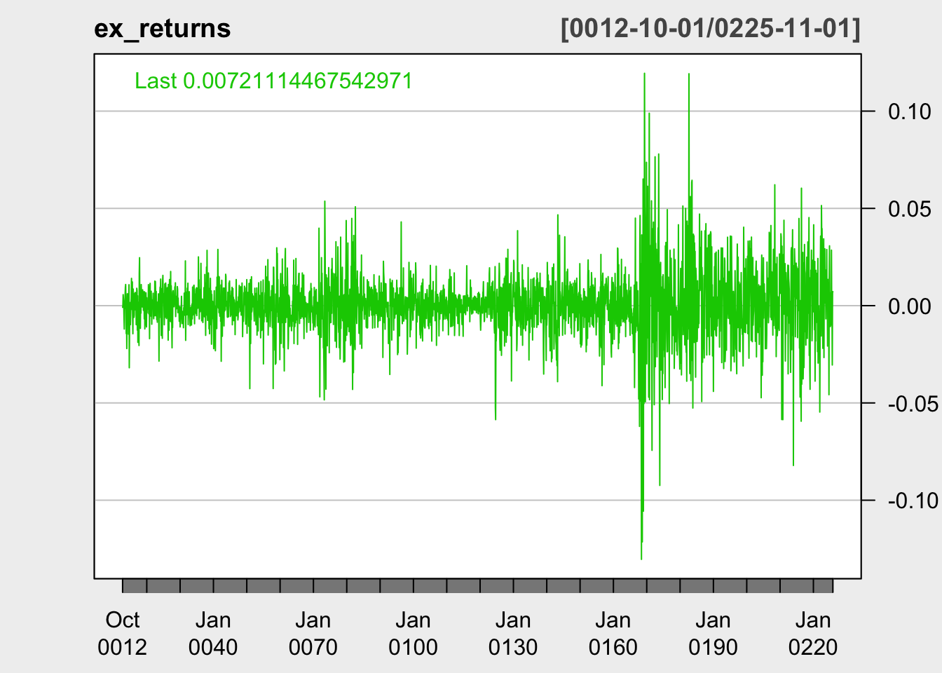
Candlestick plot of EXXON Prices over the past years, as well as the returns.
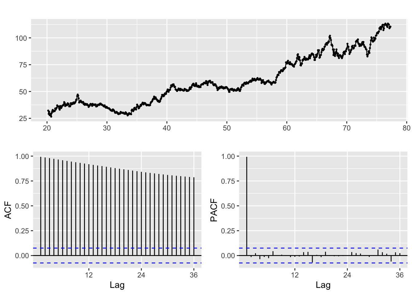
Observations: The XOM candlestick plot shows that XOM stock was between 80 and 100 USD per share between 2012 and 2018, with the exceptions of a few dips in 2016. However, the stock price has seen far more volatility in recent years, especially around 2020 and the beginning of the COVID-19 pandemic. In March 2020 the stock price plummeted to 32 USD per share, making a brief revival in June 2020 back to 50 USD per share, before dropping back to 31 USD per share in November 2020. The returns plot mirrors these findings, indicating that 2019 - 2021 saw a period of high volatility to be examined. The data appears non-stationary.
Candlestick plot of NEE Prices over the past years, as well as the returns.
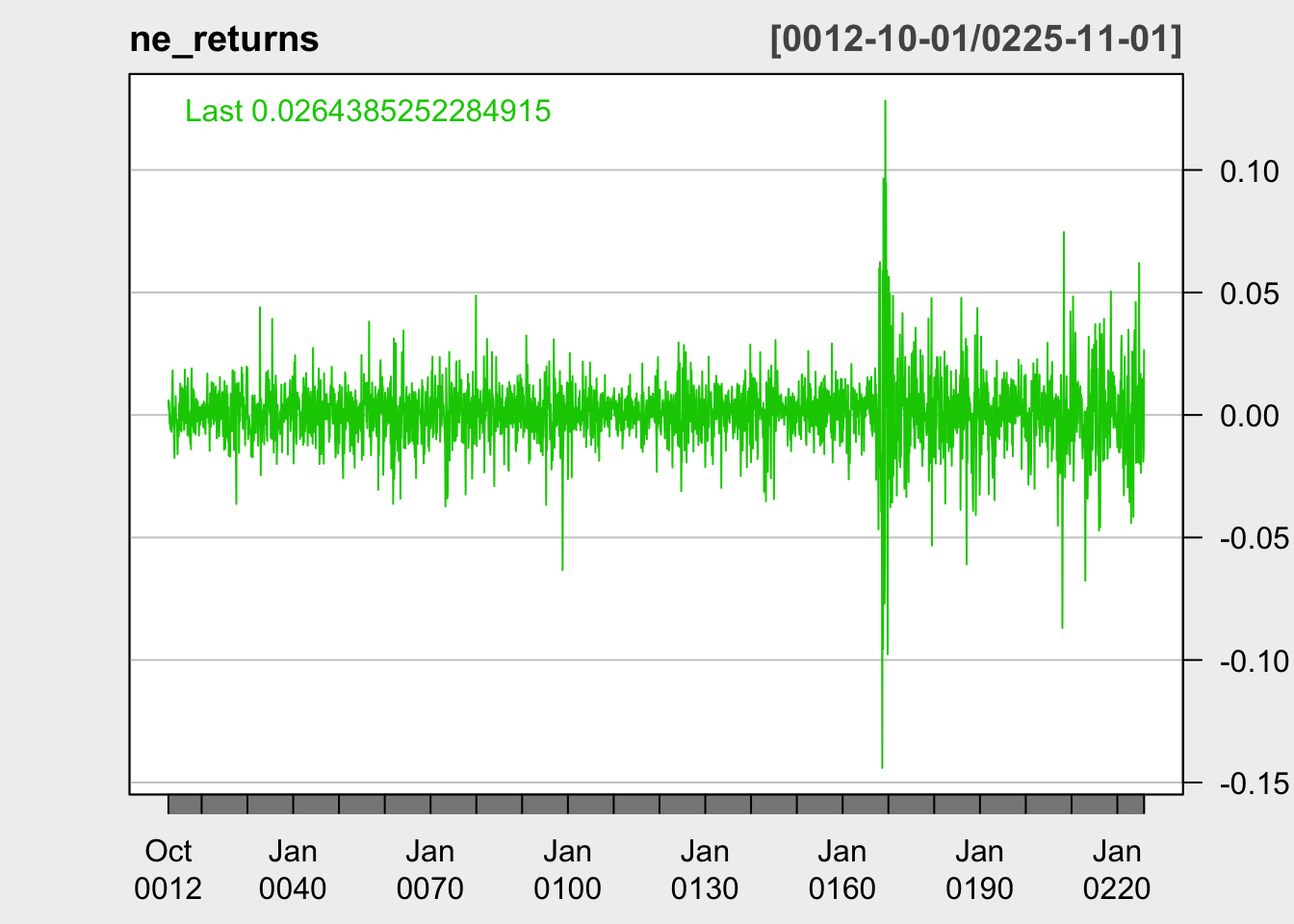
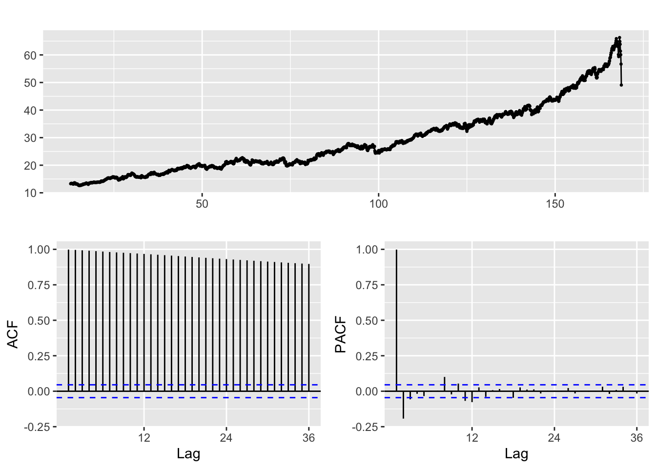
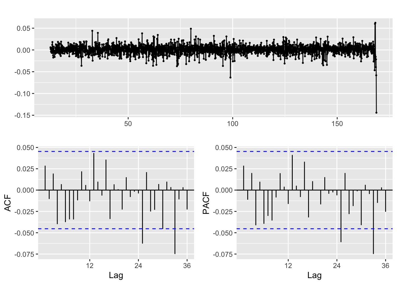
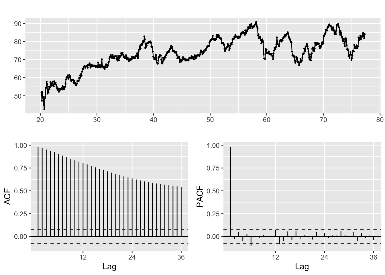
Observations: The NEE candlestick plot shows that NEE stock has steadily risen since 2012. There are some periods of volatility and stock price drops between 2020 and 2022, as the stock dropped from 67 USD to 46 USD in March 2020 and 92 USD to 73 USD between December 2021 and February 2022. The data is highly non-stationary and will need to be differenced before modeling.
Fit Model for Returns data for Exxon and Nextera Energy
Pre and post COVID 19 (March 13, 2020)
- AR+ARCH/GARCH
- ARIMA+ARCH/GARCH
1) Exxon Data
Pre-COVID 19
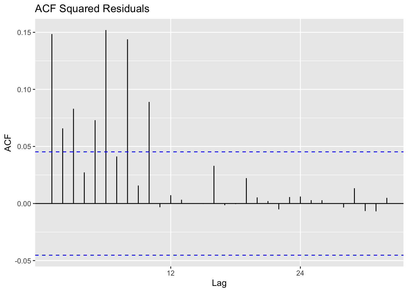
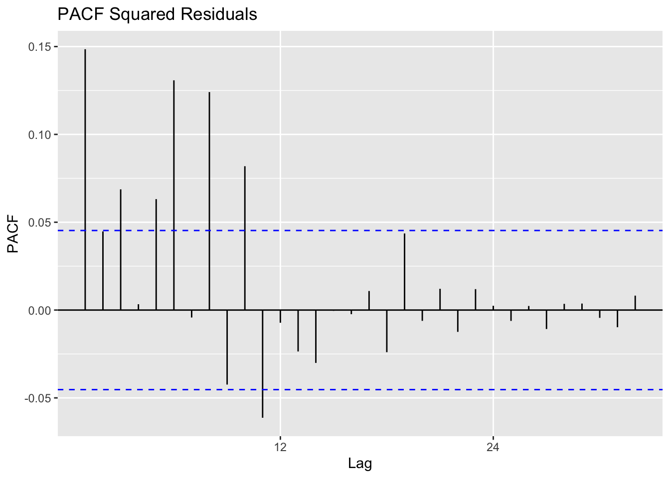
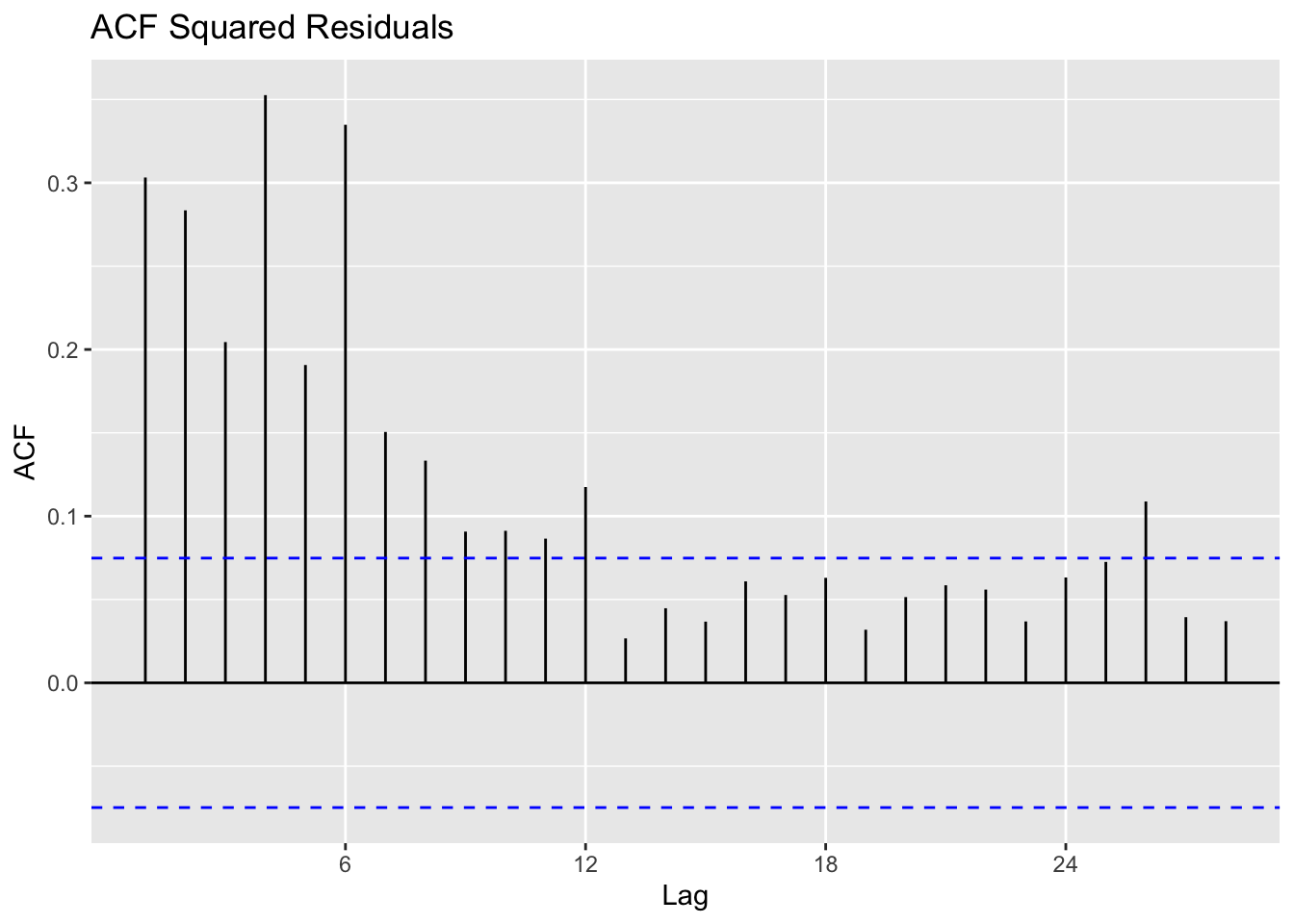
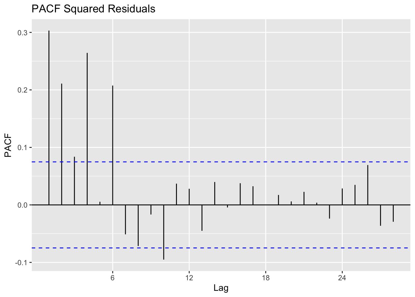
ACF/PACF plots of the returns squared
Used to determine if there are any remaining dependence structures not captured by ARCH/GARCH models.
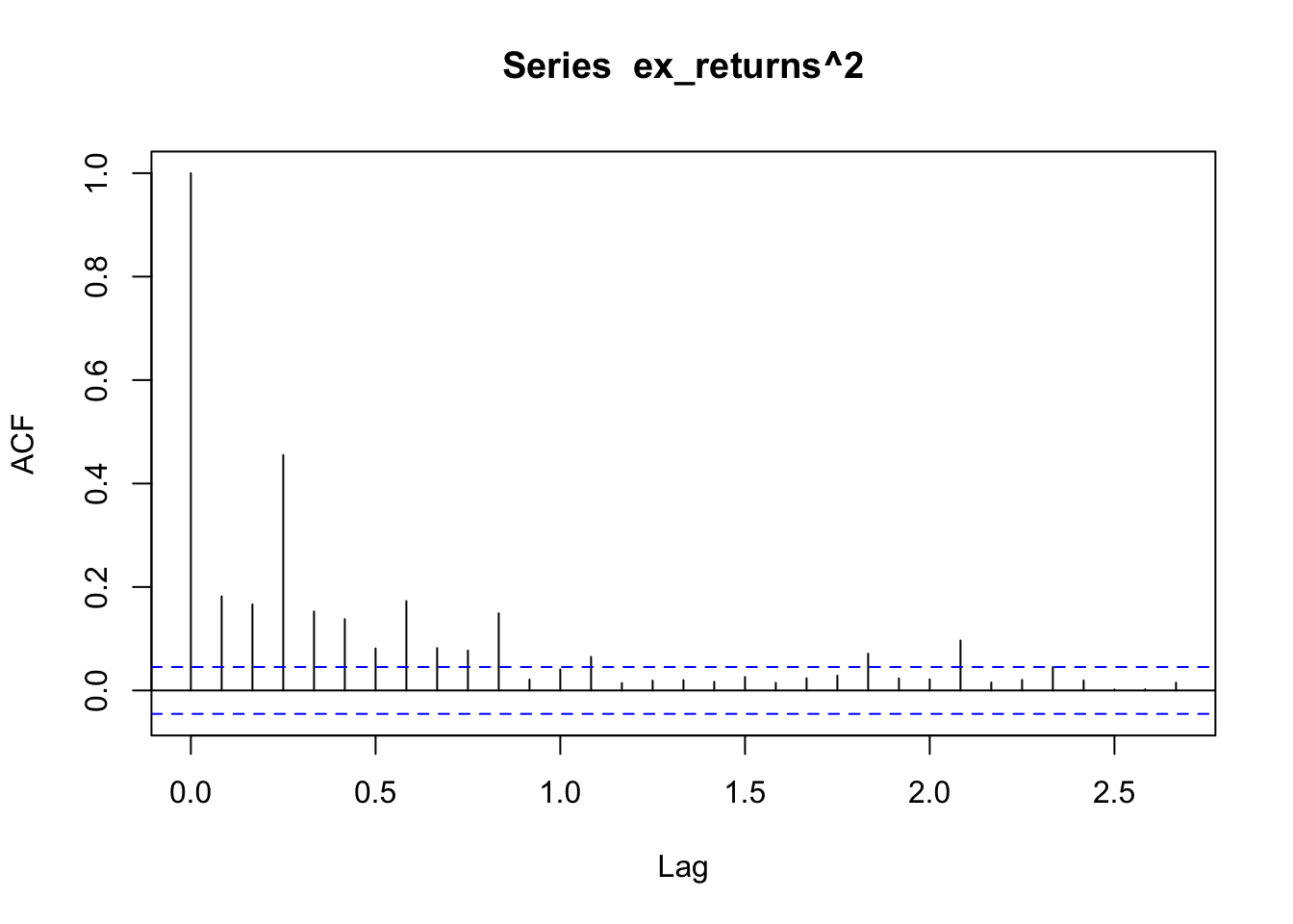
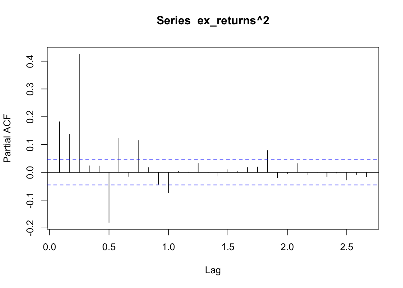
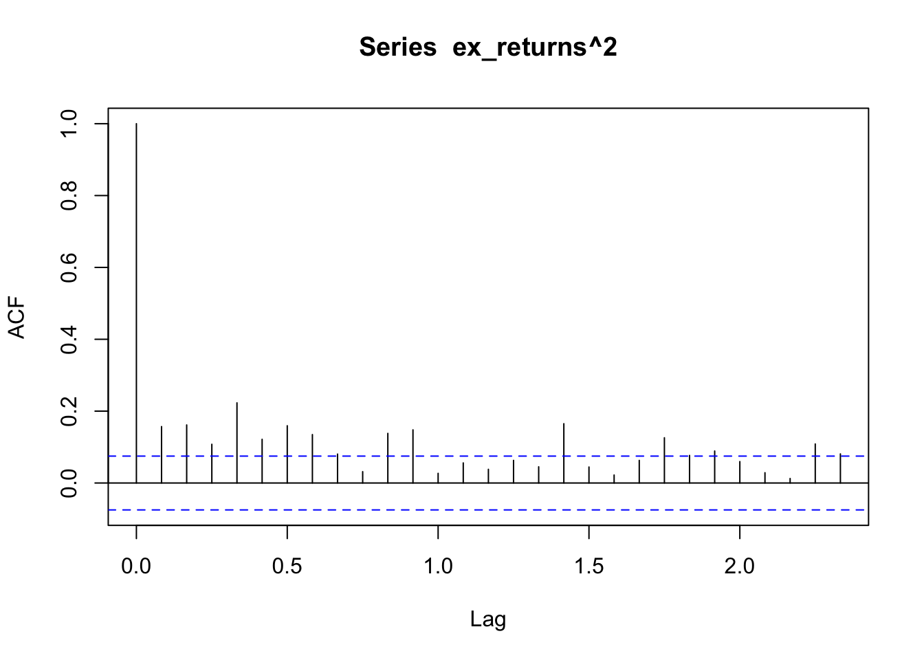
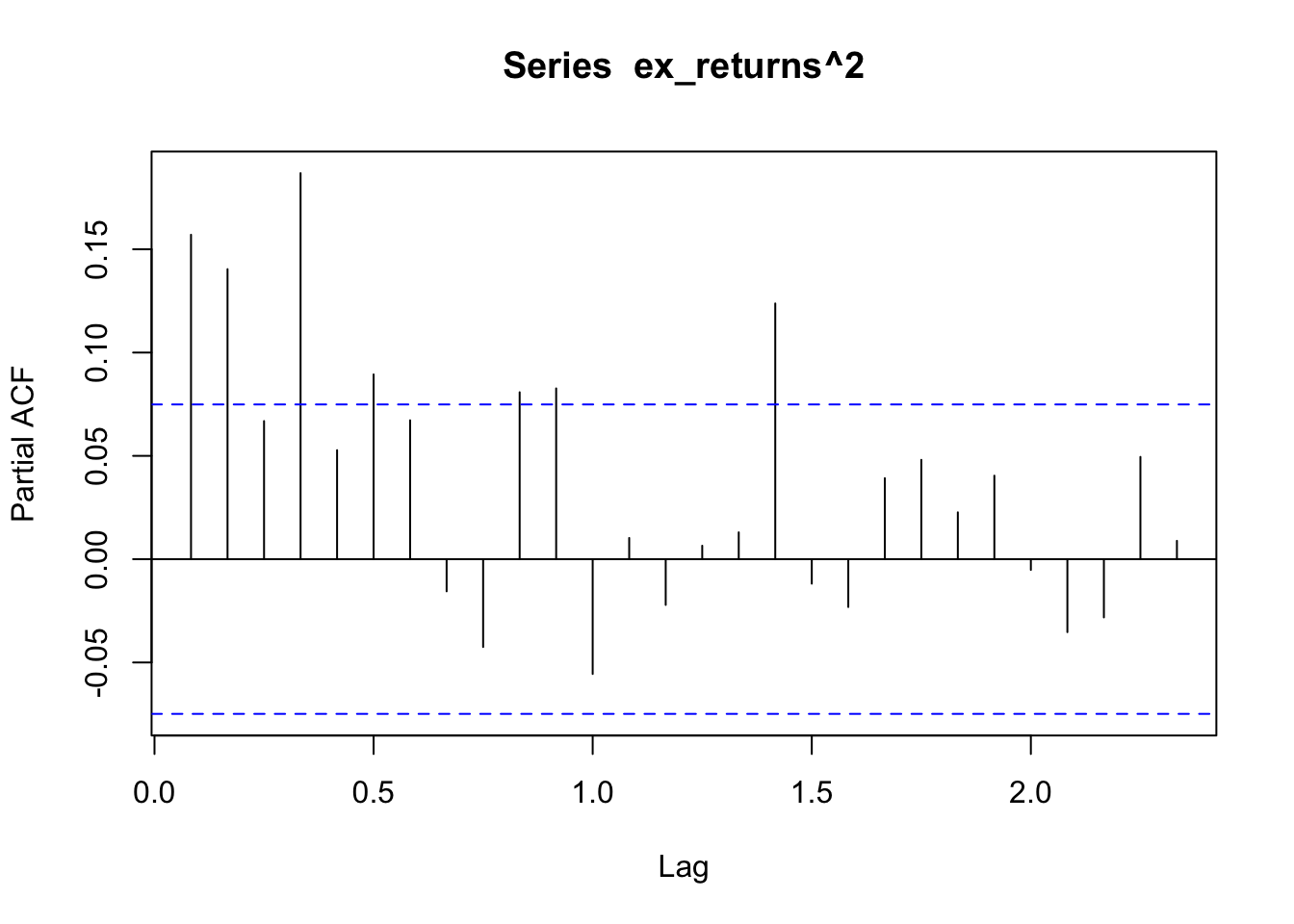
The ACF/PACF plot of returns(^2) help determine if ARCH is sufficient, or whether an AR/ARIMA model needs to be fit. From the ACF plot, I can observe that lags 0-1.0 are correlated with the time series. From the PACF plot I can observe that lags 0-1.0 are again correlated with the time series. Because there are still significant lags on both plots, an ARIMA model should be fitted first and an ARCH model can be fitted to the residuals of the ARIMA model.
Fit ARIMA model to original data
a) Check if original data is stationary
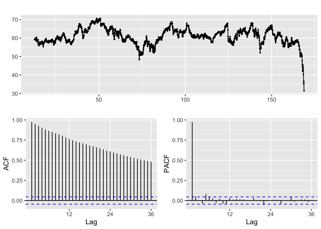
    Augmented Dickey-Fuller Test

data:  ts.exxon
Dickey-Fuller = -0.7879, Lag order = 12, p-value = 0.9627
alternative hypothesis: stationary
Exxon data is not quite stationary, as seen from the ACF/PACF plots and ADF test shown above. Thus, to make the data stationary the log of Exxon Adjusted Closing Price is taken, and differencing is undertaken.
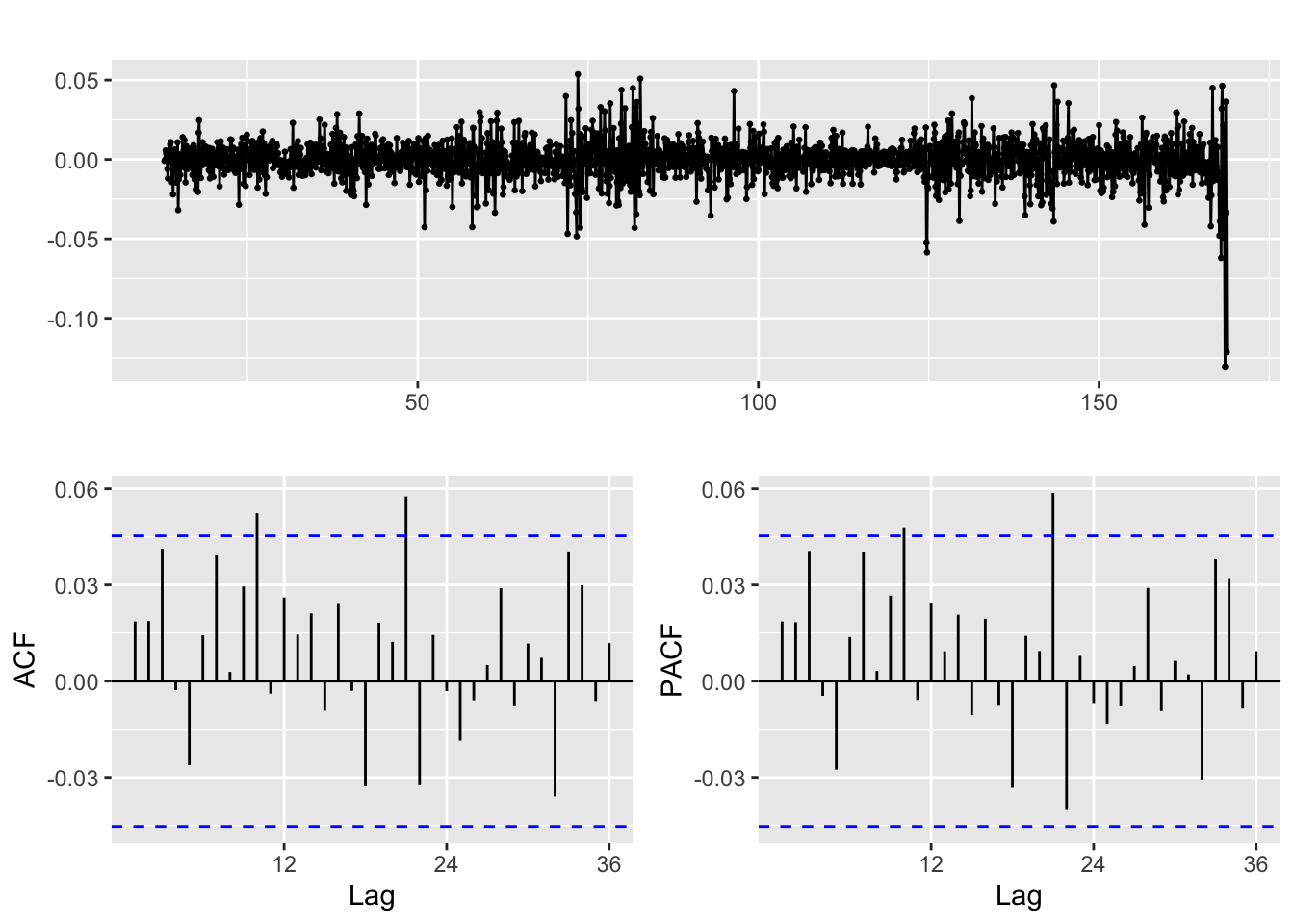
    Augmented Dickey-Fuller Test

data:  log.exxon %>% diff()
Dickey-Fuller = -8.5372, Lag order = 12, p-value = 0.01
alternative hypothesis: stationary
Just taking the log of EXXON stock data is not enough…the p-value of the ADF test is still 0.94, indicating that the data remains non-stationary. After differencing the data once, stationarity is achieved.
b) Choose p,q,d values
From the above ACF/PACF plots, values of p and q are chosen to investigate.
Moving average order (found from ACF): q - 0-24
Autoregressive term (found from pACF): p - 0-6
c) Model diagnostics
Note: There are 144 unique combinations of parameters so only the head of the resulting dataframe is shown.
| p | d | q | AIC | BIC | AICc |
|---|---|---|---|---|---|
| 0 | 1 | 0 | -11100.79 | -11089.72 | -11100.79 |
| 0 | 1 | 1 | -11099.45 | -11082.85 | -11099.44 |
| 0 | 1 | 2 | -11098.05 | -11075.91 | -11098.03 |
| 0 | 1 | 3 | -11099.52 | -11071.85 | -11099.49 |
| 0 | 1 | 4 | -11097.58 | -11064.37 | -11097.53 |
| 0 | 1 | 5 | -11096.97 | -11058.23 | -11096.91 |
Minimum AIC,BIC,and AICc
Thus, the ARIMA model that minimizes AIC and AICc is ARIMA(3,1,3).
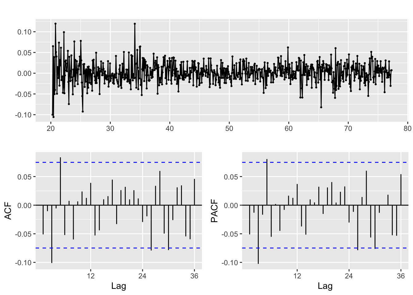
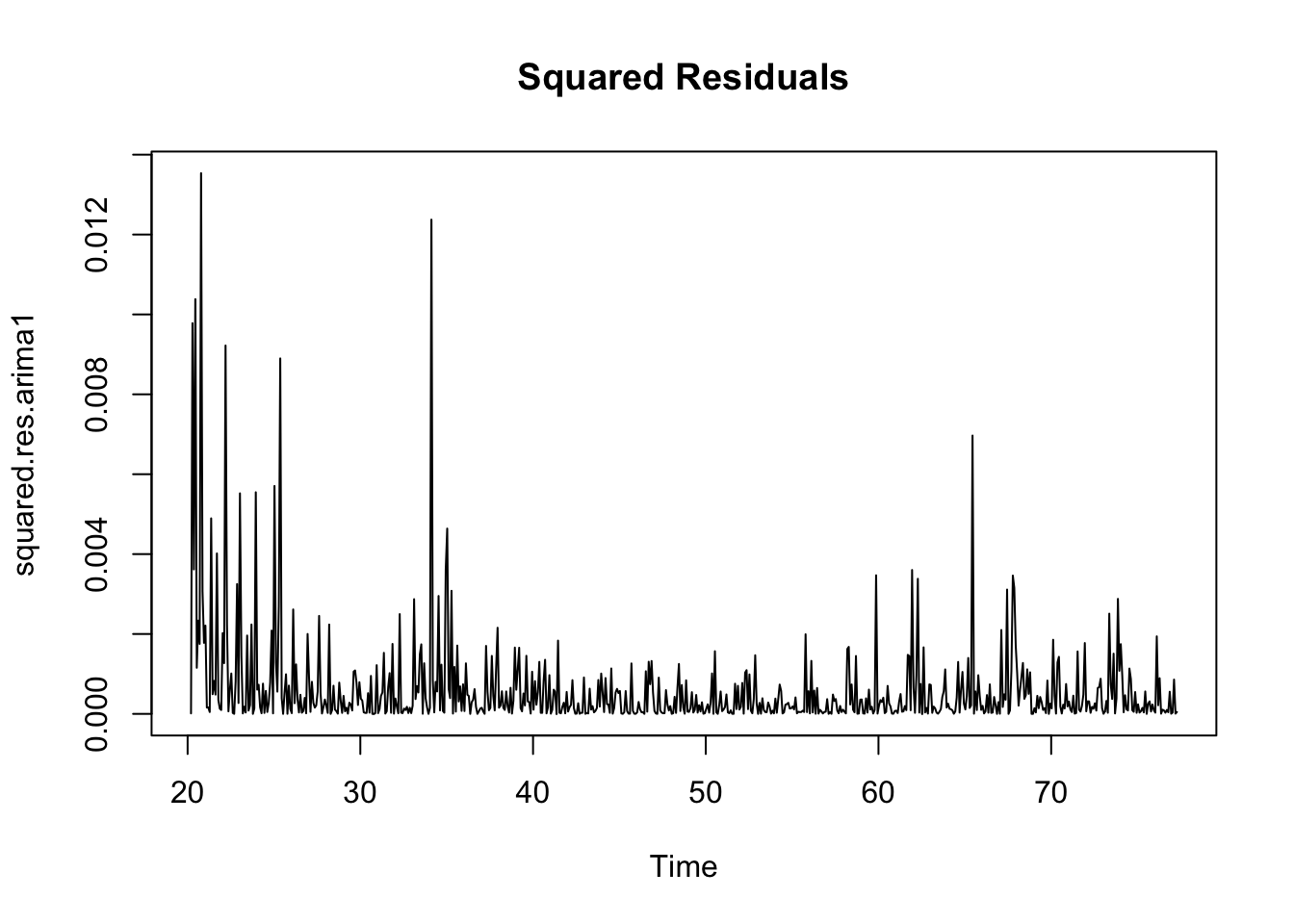
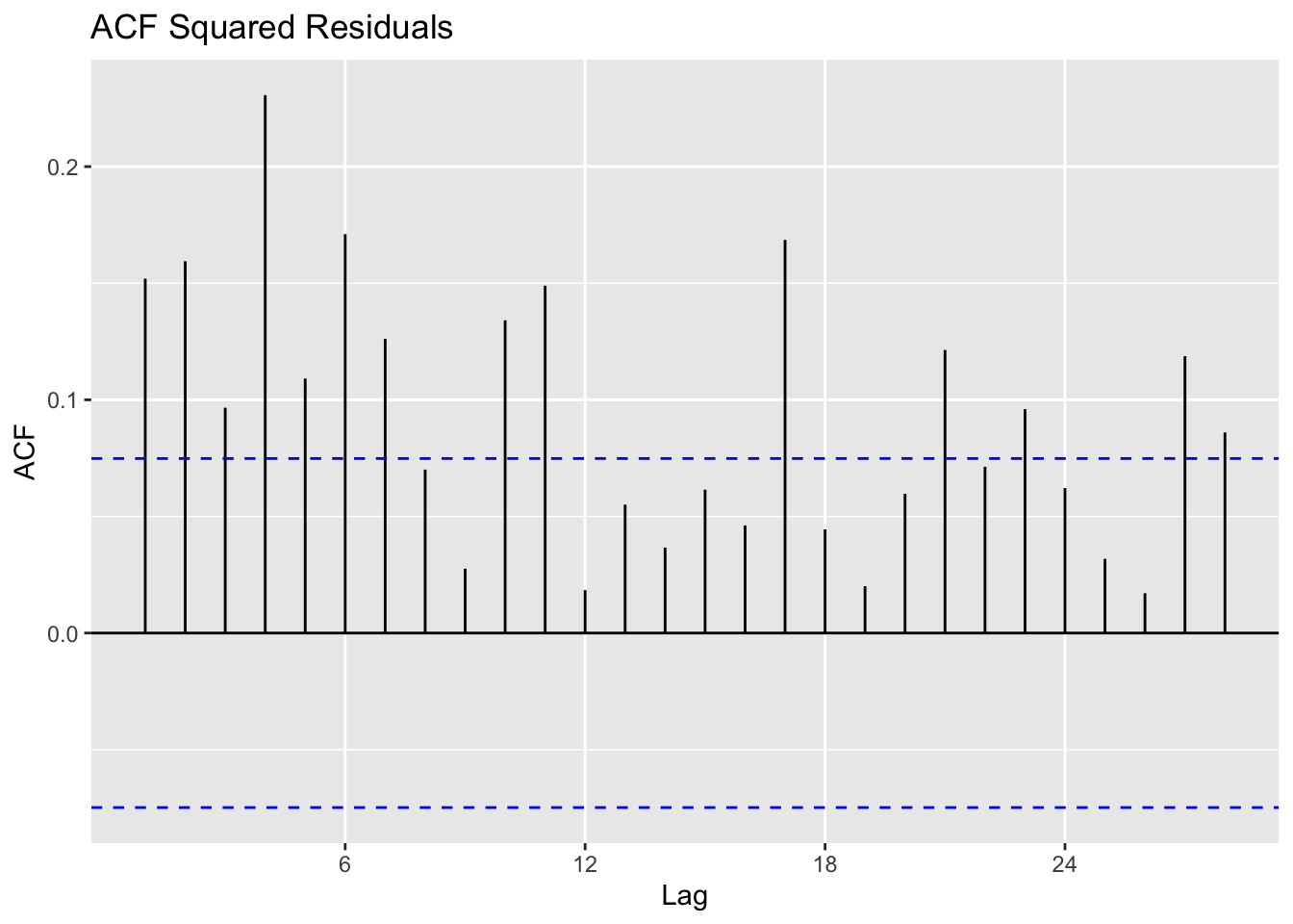
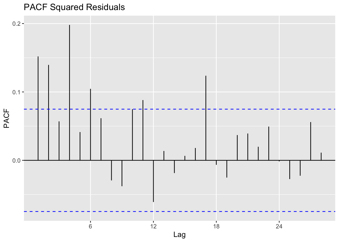
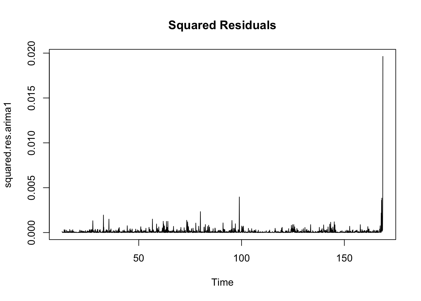
Calculate residuals of ARIMA model
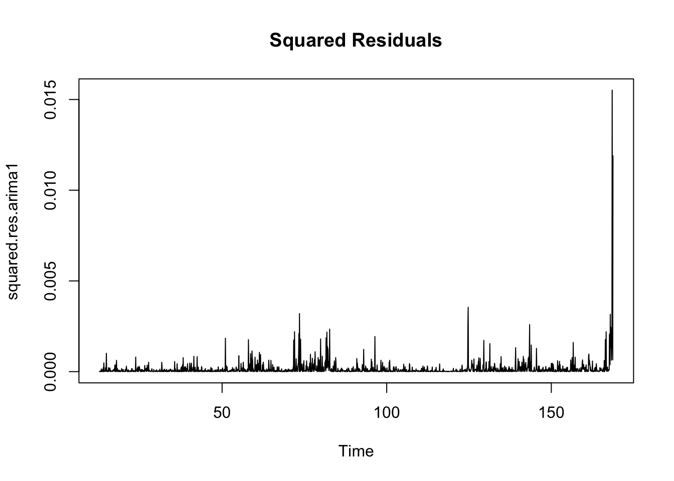
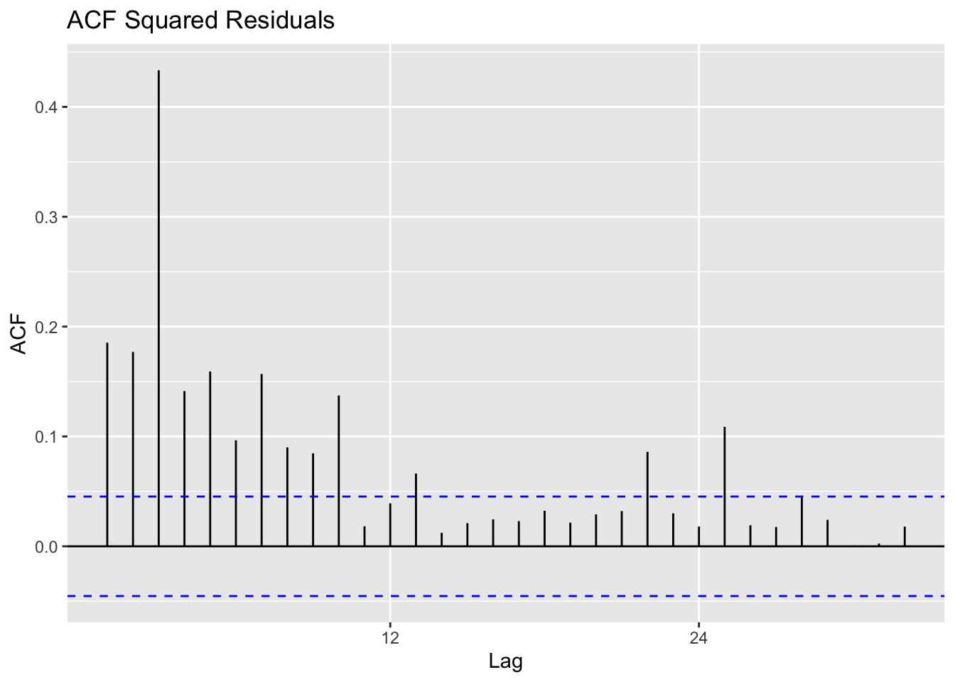
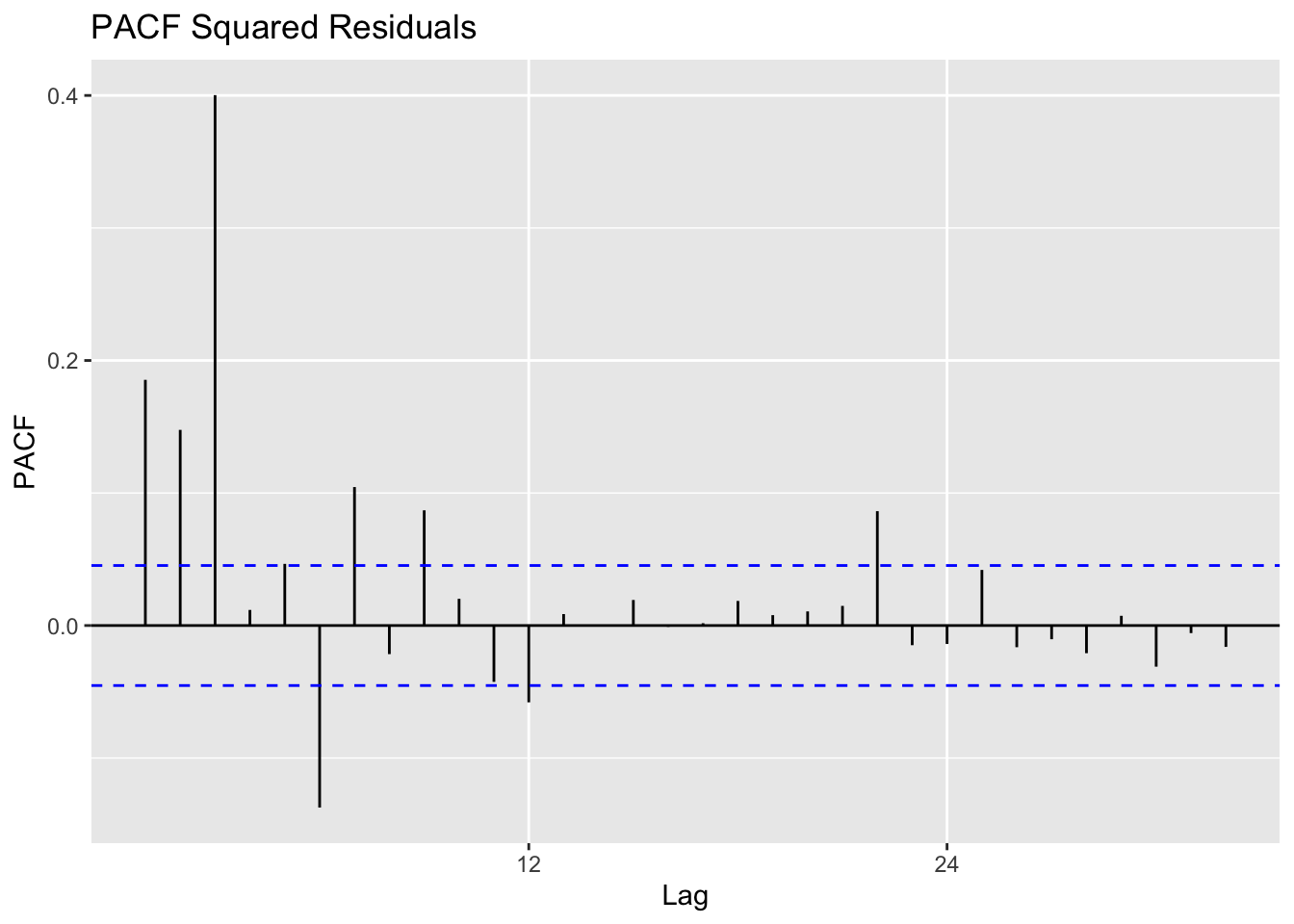
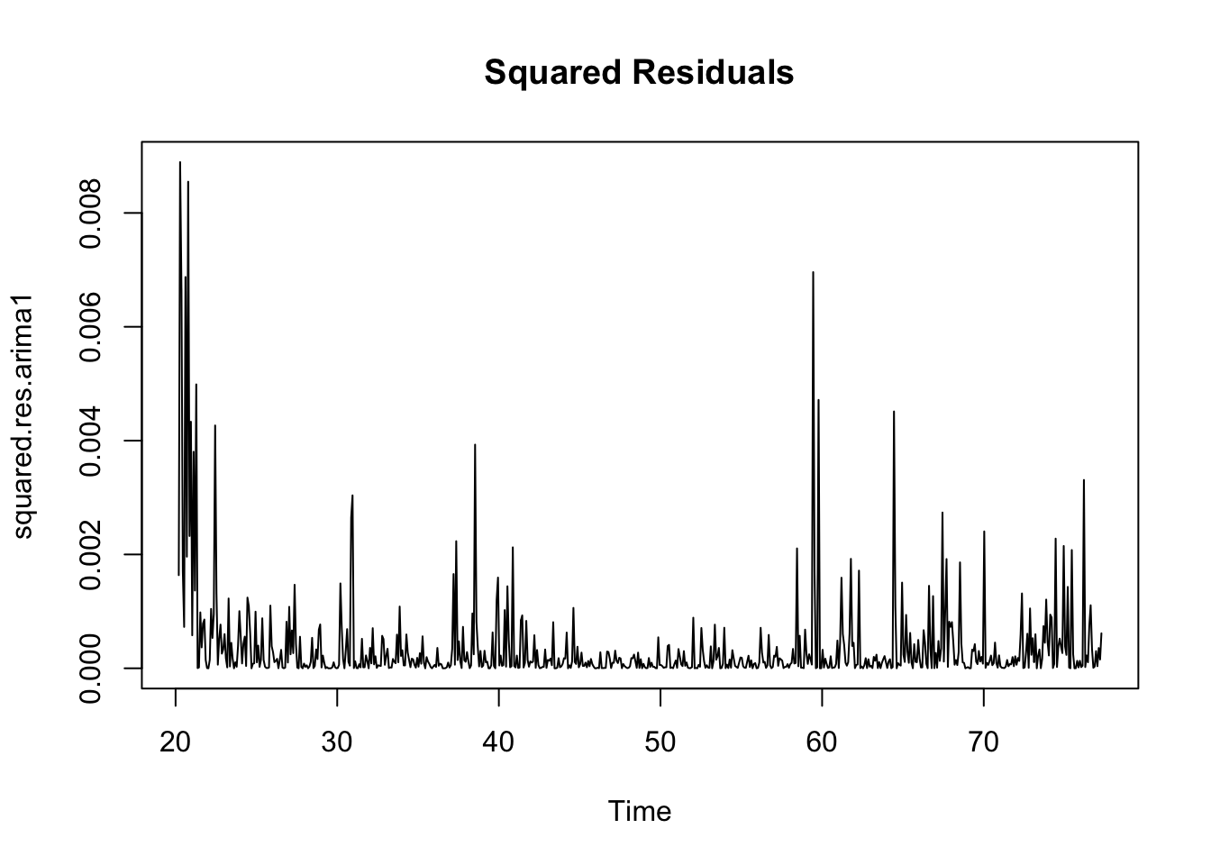
Observations: The squared residuals plot shows a cluster of volatility, while the ACF and PACF still sees significant spikes at lags 1 - 24. Thus, the residuals show that there are still some patterns that need to be modeled by ARCH/GARCH models. These methods are useful in modeling the conditional variance of the series - I try ARCH(1) through ARCH(24).
Fit ARCH models and do model diagnostics
I fit a series of GARCH models on the residuals of the ARIMA model, using parameters 0 - 10, and comparing the AIC between them.
Optimal ARCH order: 3MIN AIC: -11580.36It looks like ARCH(3) on the residuals of ARIMA(3,1,3) produces the lowest AIC and is therefore the optimal ARIMA+ARCH model. It has an AIC value of -11580.37. The model equation is below, and I look to the Box Ljung test to ensure that the model adequately represents the residuals. The Box Ljung test returns a p-value of 0.6085, so we can conclude that the model is a good fit.
    Box-Ljung test

data:  Squared.Residuals
X-squared = 0.26233, df = 1, p-value = 0.6085
Model Equation for ARIMA(3,1,3) + ARCH(3)
\[
\phi(B)x_t = \delta + \theta(B)y_t
\]
Where
\[ \phi(B) = 1 - 0.3677(B) + 0.4266(B^2) - 0.9518(B^3) \]
\[ \theta(B) = 1 - 0.8547(B) - 0.1718(B^2) + 0.9091(B^3) \]
\[ yt = \sigma_t\epsilon_t \]
\[ \begin{aligned} var(y_t|y_{t-1}) = 6.284e^{-5} + 2.063e^{-1}(y_{t-1})^2 + 2.154e^{-1}(y_{t-2})^2 + 1.618e^{-1}(y_{t-3})^2 \end{aligned} \]
Post COVID 19
ACF/PACF plots of the returns squared
Used to determine if there are any remaining dependence structures not captured by ARCH/GARCH models.
The ACF/PACF plot of returns(^2) help determine if ARCH is sufficient, or whether an AR/ARIMA model needs to be fit. From the ACF plot, I can observe that lags 0-2.0 are correlated with the time series. From the PACF plot I can observe that lags 0-2.0 are again correlated with the time series. Because there are still significant lags on both plots, an ARIMA model should be fitted first and an ARCH model can be fitted to the residuals of the ARIMA model.
Fit ARIMA model to original data
a) Check if original data is stationary
    Augmented Dickey-Fuller Test

data:  ts.exxon
Dickey-Fuller = -1.8898, Lag order = 8, p-value = 0.625
alternative hypothesis: stationary
Exxon data is certainly not stationary, as seen from the ACF/PACF plots and ADF test shown above. Thus, to make the data stationary the log of Exxon Adjusted Closing Price is taken, and differencing is undertaken.
    Augmented Dickey-Fuller Test

data:  log.exxon %>% diff()
Dickey-Fuller = -9.2086, Lag order = 8, p-value = 0.01
alternative hypothesis: stationary
Just taking the log of EXXON stock data is not enough…the p-value of the ADF test is still 0.45, indicating that the data remains non-stationary. After differencing the data once, stationarity is achieved.
b) Choose p,q,d values
From the above ACF/PACF plots, values of p,q,P,Q are chosen to investigate.
Moving average order (found from ACF): q - 1,3,5 and Q = 1,2,3
Autoregressive term (found from pACF): p - 0,1,3,5 and P = 0
c) Model diagnostics
Note: There are 98 unique combinations of parameters so only the head of the resulting dataframe is shown.
| p | d | q | P | D | Q | AIC | BIC | AICc |
|---|---|---|---|---|---|---|---|---|
| 0 | 1 | 1 | 0 | 0 | 1 | -3111.734 | -3098.145 | -3111.698 |
| 0 | 1 | 1 | 1 | 0 | 1 | -3118.084 | -3099.966 | -3118.025 |
| 0 | 1 | 1 | 0 | 0 | 2 | -3110.438 | -3092.321 | -3110.380 |
| 0 | 1 | 1 | 1 | 0 | 2 | -3116.103 | -3093.456 | -3116.015 |
| 0 | 1 | 1 | 0 | 0 | 3 | -3111.134 | -3088.487 | -3111.046 |
| 0 | 1 | 3 | 0 | 0 | 1 | -3115.274 | -3092.627 | -3115.186 |
| 1 | 1 | 1 | 0 | 0 | 1 | -3110.105 | -3091.987 | -3110.046 |
| 1 | 1 | 1 | 1 | 0 | 1 | -3117.910 | -3095.263 | -3117.822 |
| 1 | 1 | 1 | 0 | 0 | 2 | -3108.734 | -3086.087 | -3108.646 |
Minimum AIC,BIC,and AICc
Thus, the SARIMA model that minimizes AIC and AICc is SARIMA(0,1,1)(1,0,1)[12] as it minimizes AIC
Calculate residuals of ARIMA model
Observations: The squared residuals plot shows a cluster of volatility, while the ACF and PACF still sees significant spikes at lags 1 - 36. Thus, the residuals show that there are still some patterns that need to be modeled by ARCH/GARCH models. These methods are useful in modeling the conditional variance of the series - I try ARCH(1) through ARCH(24).
Fit ARCH models and do model diagnostics
I fit a series of GARCH models on the residuals of the ARIMA model, using parameters 0 - 24, and comparing the AIC between them.
Optimal ARCH order: 5MIN AIC: -3197.526It looks like ARCH(5) on the residuals of SARIMA(0,1,1)(1,0,1)[12] produces the lowest AIC and is therefore the optimal ARIMA+ARCH model. It has an AIC value of -3197.56. The model equation is below, and I look to the Box Ljung test to ensure that the model adequately represents the residuals. The Box Ljung test returns a p-value of 0.9506 so we can conclude that the model is a good fit.
    Box-Ljung test

data:  Squared.Residuals
X-squared = 0.0038361, df = 1, p-value = 0.9506
Model Equation for SARIMA(0,1,1)(1,0,1)[12] + ARCH(5)
\[
\phi(B)x_t = \delta + \theta(B)y_t
\]
Where
\[ \phi(B) = 1 + 0.9065(B^{12}) \]
\[ \theta(B) = (1 - 0.0433(B))(1 - 0.9691(B^{12})) \]
\[ yt = \sigma_t\epsilon_t \]
\[ \begin{aligned} var(y_t|y_{t-1}) = 2.963e^{-4} + 2.484e^{-2}(y_{t-1})^2 + 7.501e^{-2}(y_{t-2})^2 \\ + 1.241e^{-1}(y_{t-3})^2 + 1.608e^{-1}(y_{t-4})^2 + 9.024e^{-2}(y_{t-5})^2 \end{aligned} \]
Given the different behavior of the Exxon stock before and after the start of the COVID-19 pandemic, it is important to model the stock data separarately. The Exxon stock is far more volatile after COVID-19, whereas before the pandemic is was a bit more stable, with only a few dramatic drops in the stock price in 2015, 2018, and then 2020. Since the pandemic, Exxon stock has been rising again but has been volatile.
2) NEE Data
Pre-COVID-19
ACF/PACF plots of the returns squared
Used to determine if there are any remaining dependence structures not captured by ARCH/GARCH models.
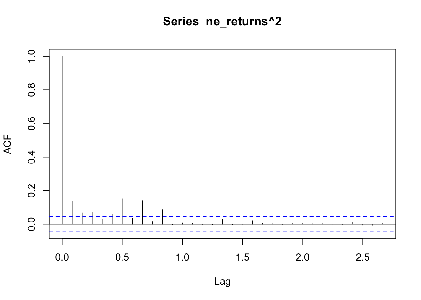
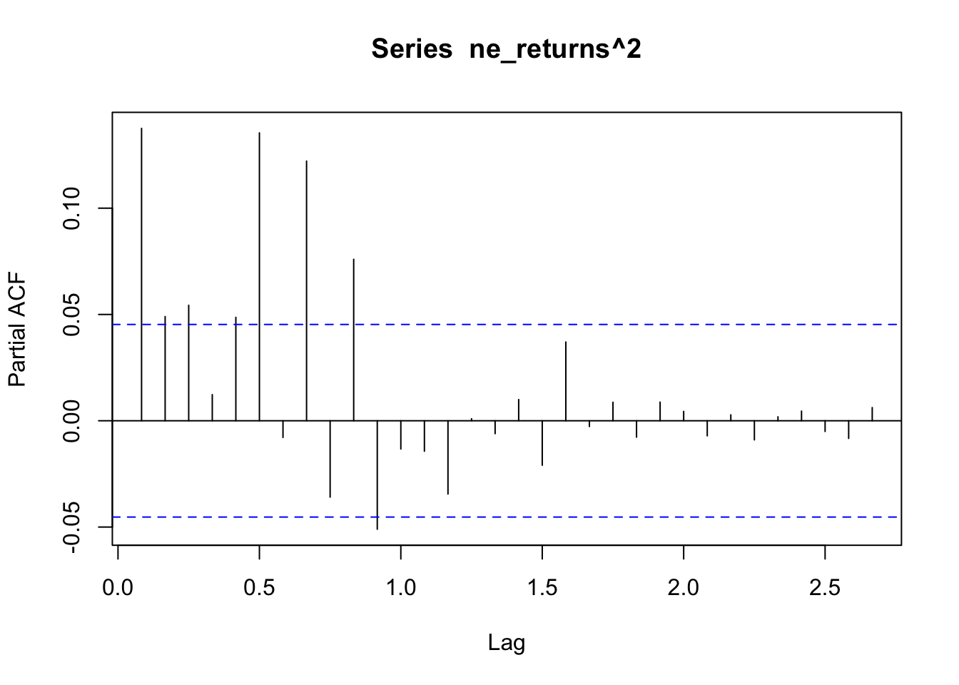
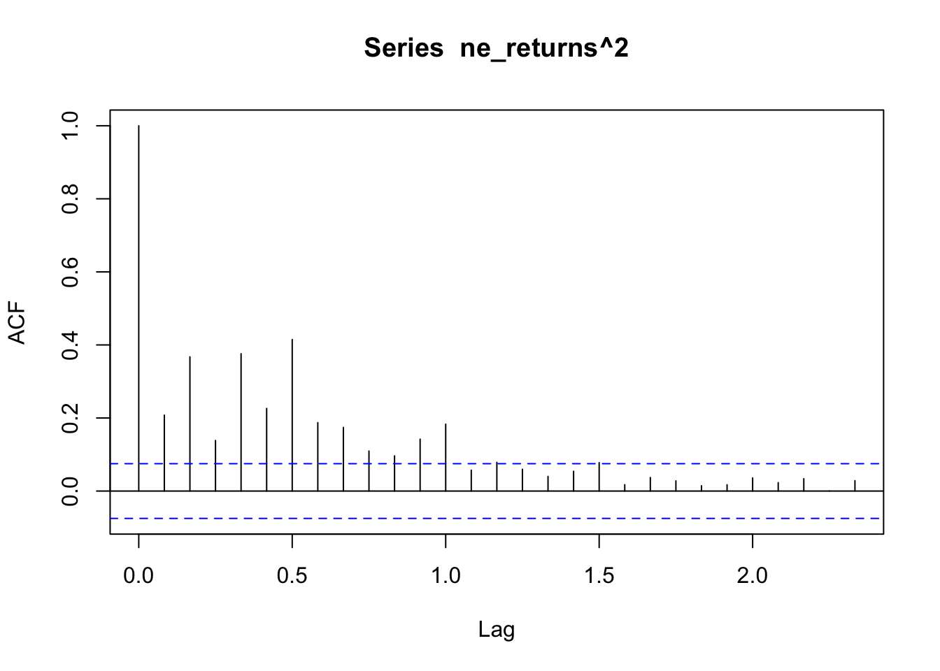
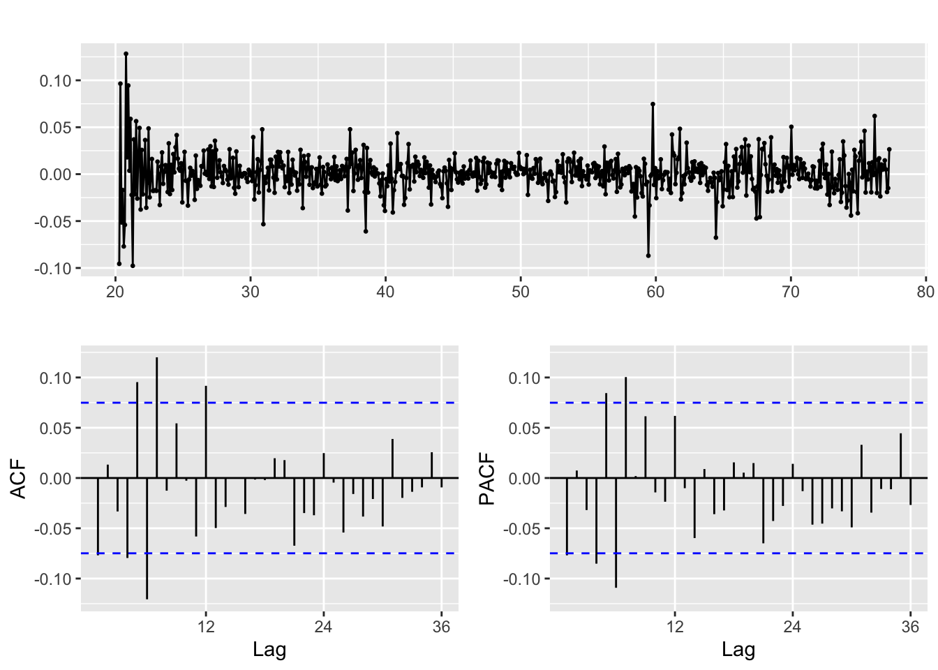
The ACF/PACF plot of returns(^2) help determine if ARCH is sufficient, or whether an AR/ARIMA model needs to be fit. From the ACF plot, I can observe that lags 0-1.5 are correlated with the time series. From the PACF plot I can observe that lags 0-1.0 are again correlated with the time series. Because there are still significant lags on both plots, an ARIMA model should be fitted first and an ARCH model can be fitted to the residuals of the ARIMA model.
Fit ARIMA model first to original data
a) Check if original data is stationary
    Augmented Dickey-Fuller Test

data:  ts.nee
Dickey-Fuller = -2.4774, Lag order = 12, p-value = 0.3762
alternative hypothesis: stationary
NEE data is not stationary, as seen from the ACF/PACF plots and ADF test shown above. Thus, to make the data stationary the log of Nee Adjusted Closing Price is taken. A drift term is also included in this analysis.
    Augmented Dickey-Fuller Test

data:  log.nee
Dickey-Fuller = -3.3, Lag order = 12, p-value = 0.07067
alternative hypothesis: stationary
Just taking the log of NEE stock data results in a p-value of the ADF test of 0.03591 Thus, we could potentially difference again or not - this will be tested during model validation. The ACF/PACF plots of the logged and first differenced NEE stock data is shown above to assist with choosing p and q values.
b) Choose p,q,d values
From the above ACF/PACF plots, values of p and q are chosen to investigate.
Moving average order (found from ACF): q - 1-6
Autoregressive term (found from pACF): p - 1-6
c) Model diagnostics
Note: There are 72 unique combinations of parameters so only the head of the resulting dataframe is shown.
| p | d | q | AIC | BIC | AICc |
|---|---|---|---|---|---|
| 0 | 0 | 0 | -4970.093 | -4953.487 | -4970.080 |
| 0 | 1 | 0 | -11601.901 | -11590.831 | -11601.894 |
| 0 | 0 | 1 | -7169.926 | -7147.785 | -7169.905 |
| 0 | 1 | 1 | -11601.635 | -11585.031 | -11601.622 |
| 0 | 0 | 2 | -8544.242 | -8516.566 | -8544.210 |
| 0 | 1 | 2 | -11599.894 | -11577.755 | -11599.873 |
Minimum AIC and AICc
Thus, the ARIMA model that minimizes AIC and AICc is ARIMA(3,0,3).
Calculate residuals of ARIMA model
Observations: The squared residuals plot shows a cluster of volatility, while the ACF and PACF still sees significant spikes at lags 0 - 12. Thus, the residuals show that there are still some patterns that need to be modeled by ARCH/GARCH models. These methods are useful in modeling the conditional variance of the series - I try ARCH(1) through ARCH(12).
Fit ARCH models and do model diagnostics
Optimal ARCH order: 5MIN AIC: -11821.87It looks like ARCH(6) on the residuals of ARIMA(3,0,4) produces the lowest AIC and is therefore the optimal ARIMA+ARCH model. It has an AIC value of -15308.36. The model equation is below, and I look to the Box Ljung test to ensure that the model adequately represents the residuals. The Box Ljung test returns a p-value of 0.8419, so we can conclude that the model is a good fit.
    Box-Ljung test

data:  Squared.Residuals
X-squared = 0.095923, df = 1, p-value = 0.7568
Model Equation for ARIMA(3,0,3) + ARCH(8)
\[
\phi(B)x_t = \delta + \theta(B)y_t
\]
Where
\[ \phi(B) = 1 + 0.6137(B) - 0.7315(B^2) - 0.8621(B^3) \]
\[ \theta(B) = 1 + 1.5710(B) + 0.7989(B^2) - 0.0653(B^3) - 0.0952(B^4) \]
\[ yt = \sigma_t\epsilon_t \]
\[ \begin{aligned} var(y_t|y_{t-1}) = 1.714e^{-4} + 9.995e^{-2}(y_{t-1})^2 + 4.243e^{-2}(y_{t-2})^2 \\ + 1.033e^{-1}(y_{t-3})^2 + 5.408e^{-2}(y_{t-4})^2 + 1.177e^{-14}(y_{t-5})^2 + 1.414e^{-1}(y_{t-6})^2 \end{aligned} \]
Post COVID 19
ACF/PACF plots of the returns squared
Used to determine if there are any remaining dependence structures not captured by ARCH/GARCH models.
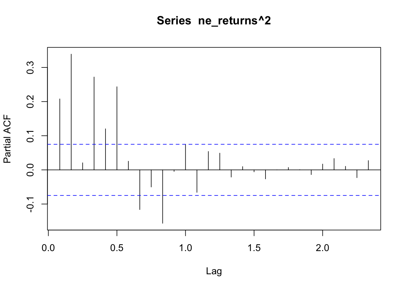
The ACF/PACF plot of returns(^2) help determine if ARCH is sufficient, or whether an AR/ARIMA model needs to be fit. From the ACF plot, I can observe that lags 0-1.0 are correlated with the time series. From the PACF plot I can observe that lags 0-1.0 are again correlated with the time series. Because there are still significant lags on both plots, an ARIMA model should be fitted first and an ARCH model can be fitted to the residuals of the ARIMA model.
Fit ARIMA model to original data
a) Check if original data is stationary
    Augmented Dickey-Fuller Test

data:  ts.nee
Dickey-Fuller = -3.544, Lag order = 8, p-value = 0.03807
alternative hypothesis: stationary
NEE data is not stationary, as seen from the ACF/PACF plots and ADF test shown above. Thus, to make the data stationary the log of Nee Adjusted Closing Price is taken. A drift term is also included in this analysis.
    Augmented Dickey-Fuller Test

data:  log.nee
Dickey-Fuller = -3.5665, Lag order = 8, p-value = 0.03591
alternative hypothesis: stationary
Just taking the log of NEE stock data results in a p-value of the ADF test of 0.03591 Thus, we could potentially difference again or not - this will be tested during model validation. The ACF/PACF plots of the logged and first differenced NEE stock data is shown above to assist with choosing p and q values.
b) Choose p,q,d values
From the above ACF/PACF plots, values of p and q are chosen to investigate.
Moving average order (found from ACF): q - 1-8
Autoregressive term (found from pACF): p - 1-8
c) Model diagnostics
Note: There are 98 unique combinations of parameters so only the head of the resulting dataframe is shown.
| p | d | q | AIC | BIC | AICc |
|---|---|---|---|---|---|
| 0 | 0 | 0 | -1407.736 | -1394.143 | -1407.701 |
| 0 | 1 | 0 | -3419.199 | -3410.140 | -3419.181 |
| 0 | 0 | 1 | -2172.011 | -2153.888 | -2171.952 |
| 0 | 1 | 1 | -3421.326 | -3407.738 | -3421.291 |
| 0 | 0 | 2 | -2574.993 | -2552.339 | -2574.905 |
| 0 | 1 | 2 | -3419.397 | -3401.280 | -3419.339 |
Minimum AIC,BIC,and AICc
Thus, the ARIMA model that minimizes AIC and AICc is ARIMA(3,0,4) again!
Calculate residuals of ARIMA model
Observations: The squared residuals plot shows a cluster of volatility, while the ACF and PACF still sees significant spikes at lags 1 - 12. Thus, the residuals show that there are still some patterns that need to be modeled by ARCH/GARCH models. These methods are useful in modeling the conditional variance of the series - I try ARCH(1) through ARCH(12).
Fit ARCH models and do model diagnostics
I fit a series of GARCH models on the residuals of the ARIMA model, using parameters 0 - 12, and comparing the AIC between them.
Optimal ARCH order: 6MIN AIC: -3586.809It looks like ARCH(6) on the residuals of ARIMA(3,0,4) produces the lowest AIC and is therefore the optimal ARIMA+ARCH model. It has an AIC value of -3197.56. The model equation is below, and I look to the Box Ljung test to ensure that the model adequately represents the residuals. The Box Ljung test returns a p-value of 0.8419 so we can conclude that the model is a good fit.
    Box-Ljung test

data:  Squared.Residuals
X-squared = 0.098416, df = 1, p-value = 0.7537
Model Equation for ARIMA(3,0,3) + ARCH(8)
\[
\phi(B)x_t = \delta + \theta(B)y_t
\]
Where
\[ \phi(B) = 1 + 0.6137(B) - 0.7315(B^2) - 0.8621(B^3) \]
\[ \theta(B) = 1 + 1.5710(B) + 0.7989(B^2) - 0.0653(B^3) - 0.0952(B^4) \]
\[ yt = \sigma_t\epsilon_t \]
\[ \begin{aligned} var(y_t|y_{t-1}) = 1.714e^{-4} + 9.995e^{-2}(y_{t-1})^2 + 4.243e^{-2}(y_{t-2})^2 \\ + 1.033e^{-1}(y_{t-3})^2 + 5.408e^{-2}(y_{t-4})^2 + 1.177e^{-14}(y_{t-5})^2 + 1.414e^{-1}(y_{t-6})^2 \end{aligned} \] Given the different behavior of the Nextera stock before and after the start of the COVID-19 pandemic, it is important to model the stock data separarately. The Nextera stock is far more volatile after COVID-19, whereas before the pandemic is was steadily incrreasing in value between 2012-2020. Since the pandemic, though more volatile, the stock has continued to trend upwards over time.
Source code for the above analysis: Github