ARMA/ARIMA/SARIMA Models
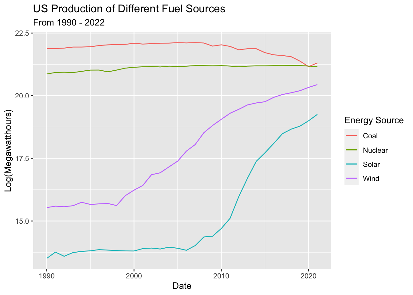
Dataset 1 - Electricity Production
1) Data Review
From EDA, we looked at ACF graphs and checked ADF to see if the data was stationary. The data was not stationary so we’ll take the log to try to make it at least weakly stationary.
Log Transform energy production outputs - and plot
Check if data is now stationary using ACF plot
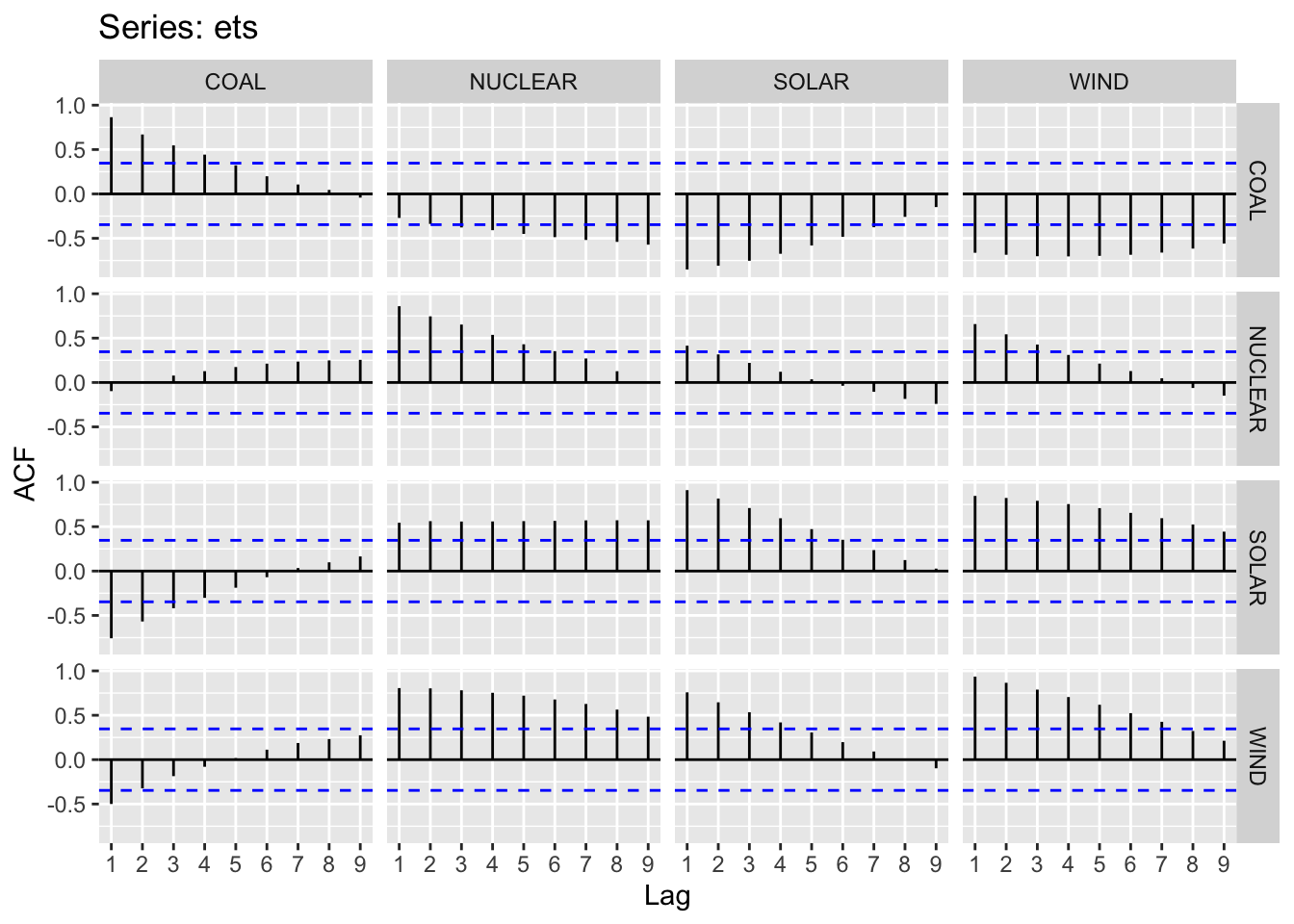
It’s now weakly stationary! No further differencing necessary.
2) ACF/PACF Plots
ACF/PACF plots are used to select potential p and q values for an ARMA(p,q) model. ARMA is used because no differencing of the data occurred. From these plots, some potential p and q values are selected to fit an ARMA model with. Separate models have to be fit for each energy source, thus separate ACF/PACF plots are shown below.
Coal
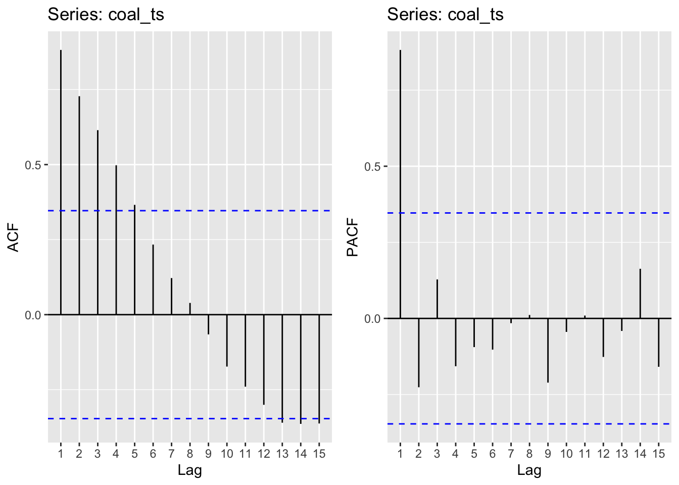
Moving average order (found from ACF): q - 1,2,3,4
Autoregressive term (found from pACF): p - 1
Nuclear
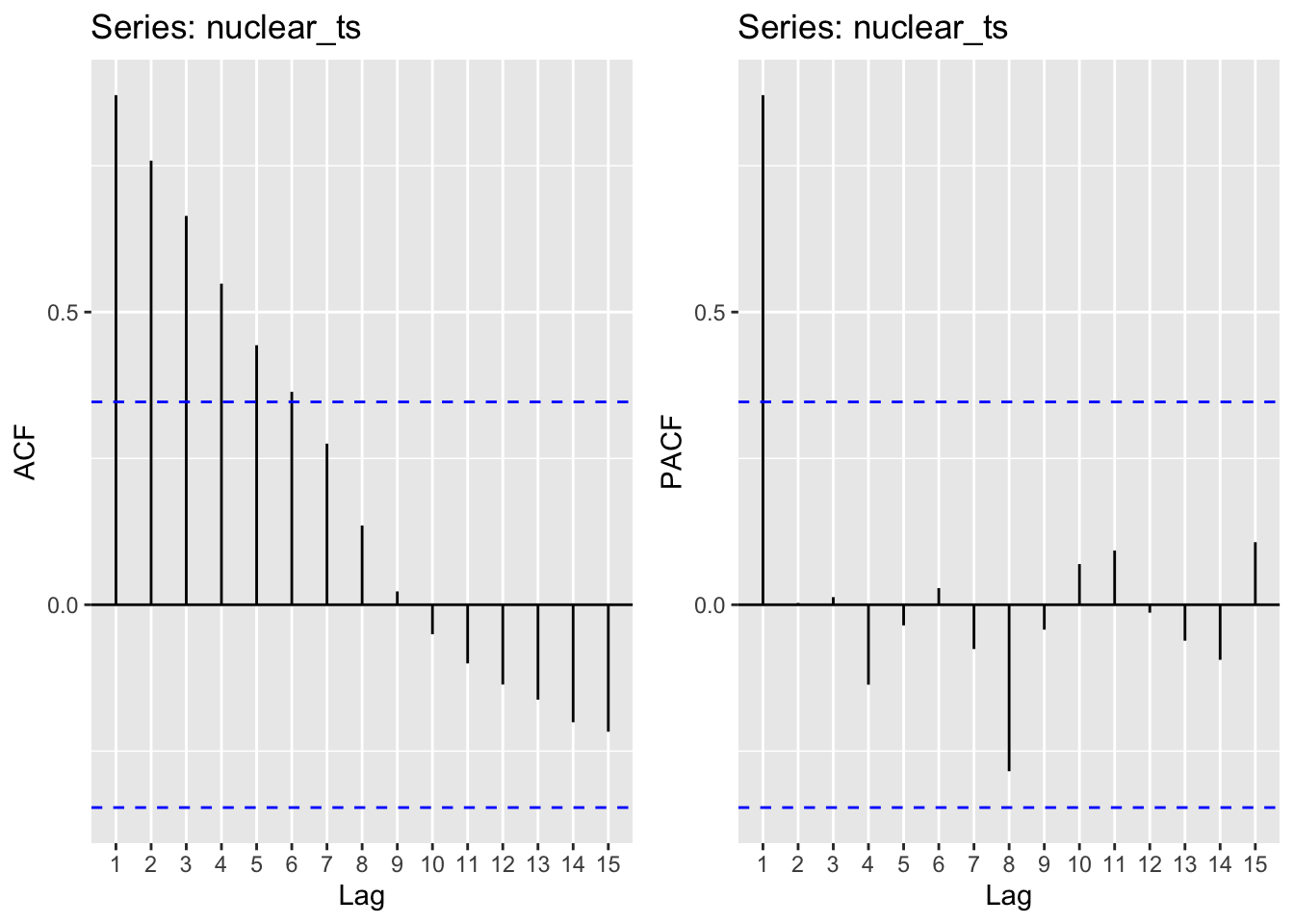
Moving average order (found from ACF): q - 1,2,3,4,5
Autoregressive term (found from pACF): p - 1
Wind
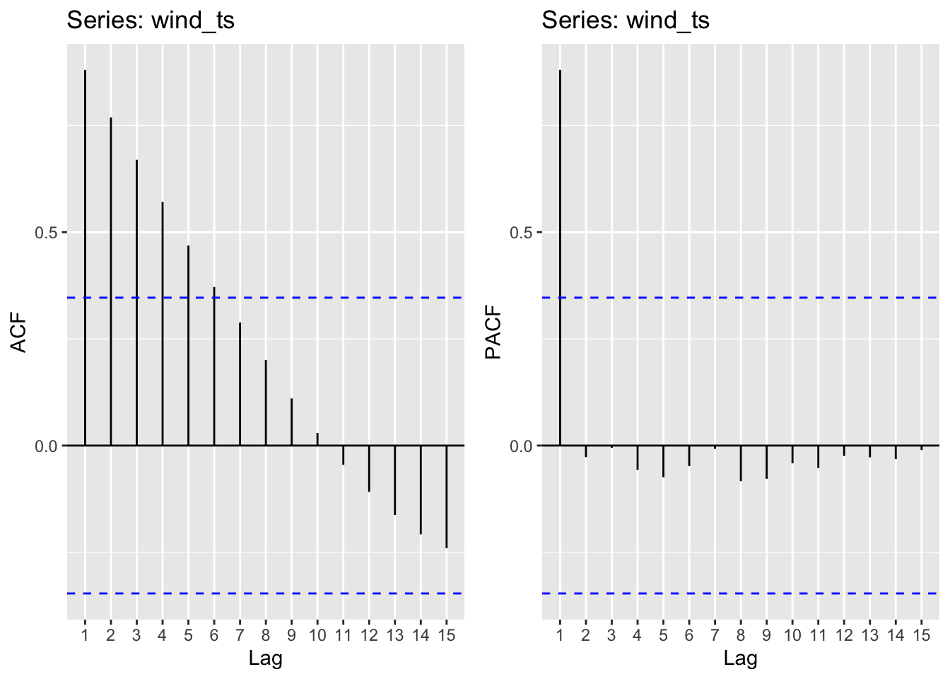
Moving average order (found from ACF): q - 1,2,3,4,5
Autoregressive term (found from pACF): p - 1
Solar
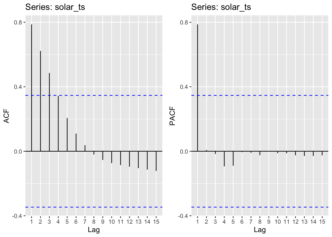
Moving average order (found from ACF): q - 1,2,3
Autoregressive term (found from pACF): p - 1
3) Fit ARIMA(p,d,q) models
Coal
| p | q | AIC |
|---|---|---|
| 1 | 1 | 1319.547 |
| 1 | 2 | 1325.199 |
| 1 | 3 | 1312.109 |
| 1 | 4 | 1313.924 |
Nuclear
| p | q | AIC |
|---|---|---|
| 1 | 1 | 1213.296 |
| 1 | 2 | 1212.388 |
| 1 | 3 | 1214.309 |
| 1 | 4 | 1225.694 |
| 1 | 5 | 1229.118 |
Wind
| p | q | AIC |
|---|---|---|
| 1 | 1 | 1144.565 |
| 1 | 2 | 1147.529 |
| 1 | 3 | 1148.876 |
| 1 | 4 | 1147.240 |
| 1 | 5 | 1150.403 |
Solar
| p | q | AIC |
|---|---|---|
| 1 | 1 | 1069.721 |
| 1 | 2 | 1063.944 |
| 1 | 3 | 1073.950 |
4) Model Diagnostics
With the above exploration, a best fit model is chosen for each energy source by minimizing AIC.
Coal
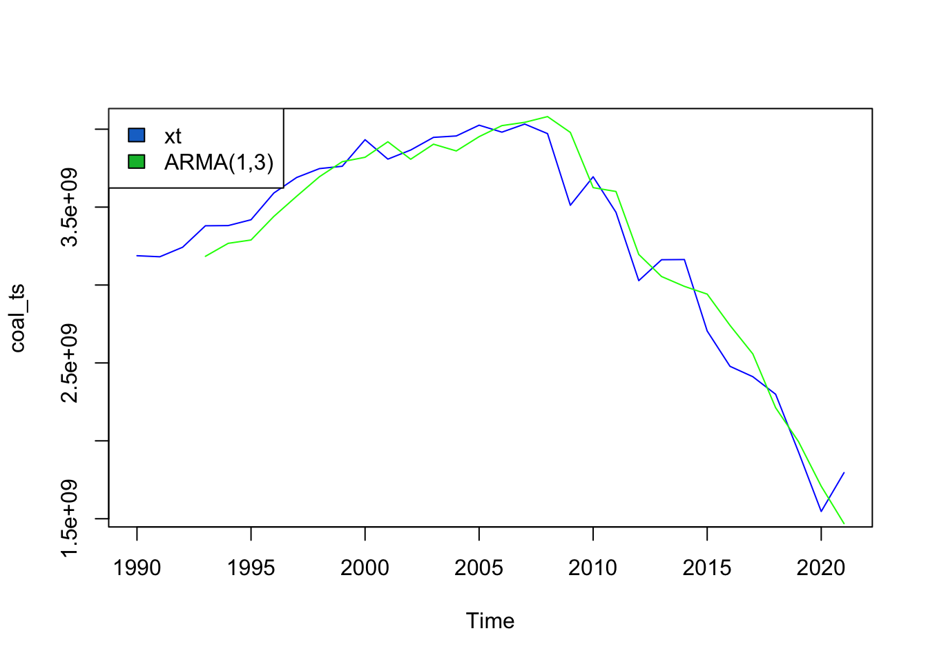
The ARMA(p,q) model that minimizes AIC is ARMA(1,3).
Call:
arma(x = coal_ts, order = c(1, 3))

Model:
ARMA(1,3)

Residuals:
       Min         1Q     Median         3Q        Max
-467564239 -111368527   52069246  112738236  326924565

Coefficient(s):
            Estimate  Std. Error    t value Pr(>|t|)
ar1        1.074e+00   9.793e-03    109.664   <2e-16 ***
ma1       -3.294e-01   2.462e-01     -1.338   0.1810
ma2       -3.552e-02   6.203e-01     -0.057   0.9543
ma3        5.782e-01   2.625e-01      2.203   0.0276 *
intercept -2.978e+08   1.120e+04 -26602.741   <2e-16 ***
---
Signif. codes:  0 '***' 0.001 '**' 0.01 '*' 0.05 '.' 0.1 ' ' 1

Fit:
sigma^2 estimated as 2.75e+16,  Conditional Sum-of-Squares = 7.701038e+17,  AIC = 1312.11
ARMA(1,3) for coal produces an AIC value of 1312.11 and a CSS value of 7.7x10^17. Using the model summary and plot of the model against the data above, it seems that the model fits the data pretty well but not perfectly. The randomness and sensitivity of the original data makes it hard for the model to truly fit well without overfitting. To achieve a better fit would require overfitting the training data and wouldn’t generalize well to new data.
\[ \phi(B) = 1 - 1.07(B) \] \[ \theta(B) = 1 + 3.29*10^-1 *(B) + 3.552*10^-2*(B^2) - 5.782*10^-1*(B^3) \]
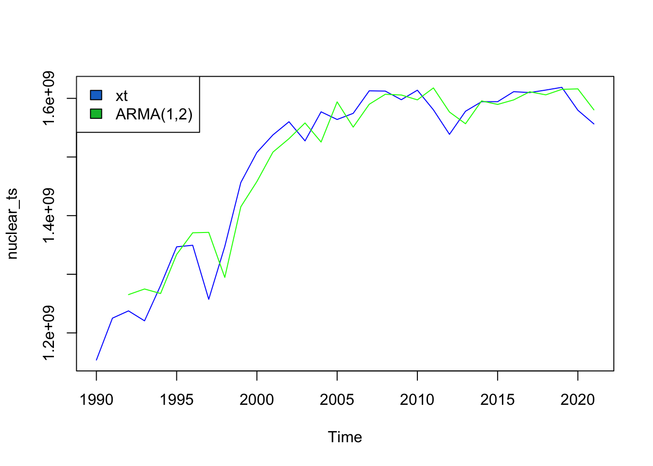
Nuclear
The ARMA(p,q) model that minimizes AIC is ARMA(1,2).
Call:
arma(x = nuclear_ts, order = c(1, 2))

Model:
ARMA(1,2)

Residuals:
       Min         1Q     Median         3Q        Max
-114143177  -26807890    5091034   22515762   52763712

Coefficient(s):
            Estimate  Std. Error   t value Pr(>|t|)
ar1        8.976e-01   3.176e-03   282.600   <2e-16 ***
ma1        5.650e-02   1.914e-01     0.295   0.7678
ma2       -3.256e-01   1.744e-01    -1.868   0.0618 .
intercept  1.657e+08   7.670e+03 21598.292   <2e-16 ***
---
Signif. codes:  0 '***' 0.001 '**' 0.01 '*' 0.05 '.' 0.1 ' ' 1

Fit:
sigma^2 estimated as 1.298e+15,  Conditional Sum-of-Squares = 3.764894e+16,  AIC = 1212.39
ARMA(1,2) for nuclear produces an AIC value of 1212.39 and a CSS value of 3.76x10^16. It seems that the model fits the data pretty well but not perfectly. To achieve a better fit would require overfitting the training data and wouldn’t generalize well to new data.
\[ \phi(B) = 1 - 8.976*10^-1(B) \] \[ \theta(B) = 1 - 5.65*10^-2 *(B) + 3.256*10^-1*(B^2) \]
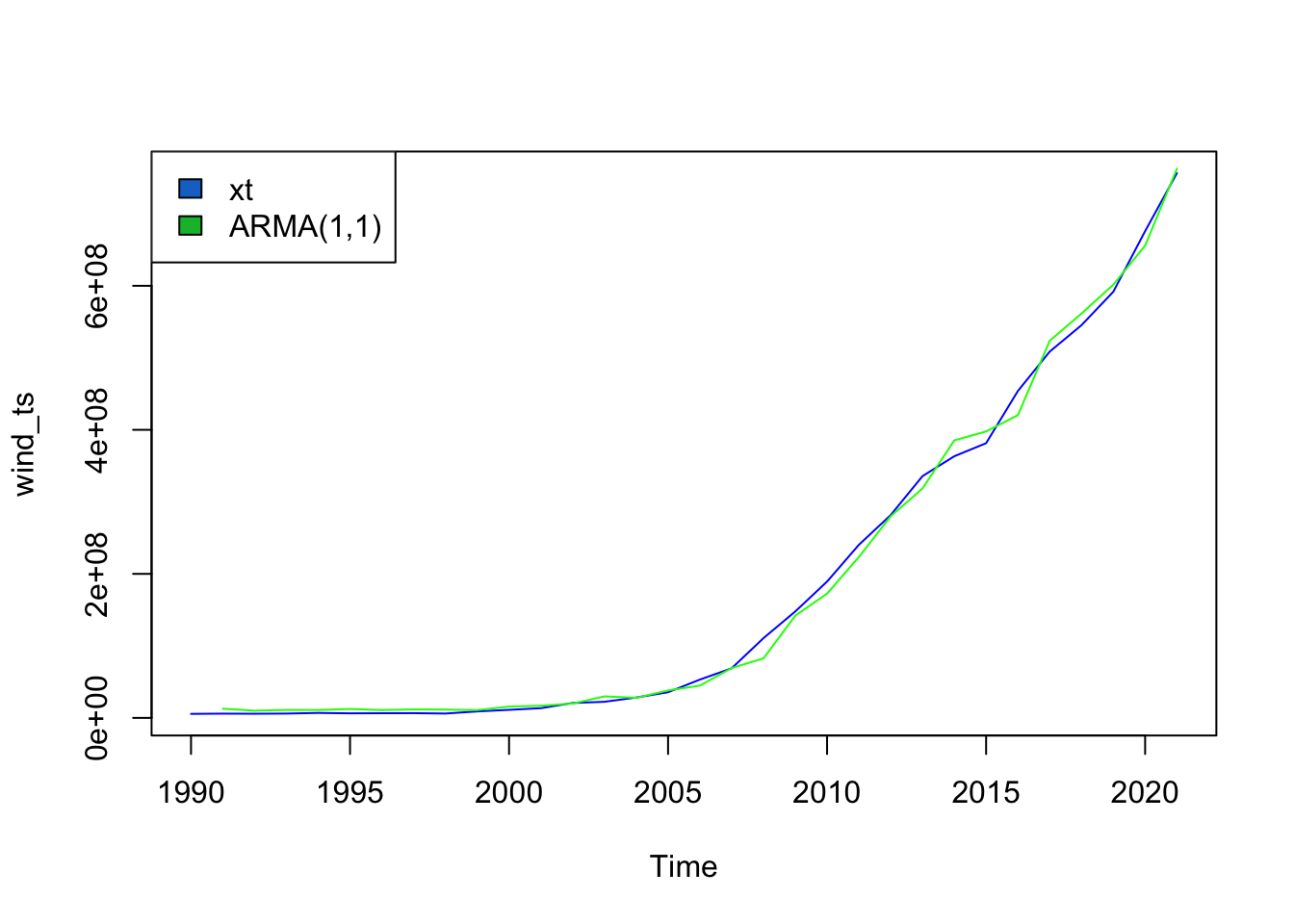
Wind
The ARMA(p,q) model that minimizes AIC is ARMA(1,1).
Call:
arma(x = wind_ts, order = c(1, 1))

Model:
ARMA(1,1)

Residuals:
      Min        1Q    Median        3Q       Max
-22040549  -6078188  -4049714   3768737  33558013

Coefficient(s):
           Estimate  Std. Error  t value Pr(>|t|)
ar1       1.105e+00   1.202e-02   91.912   <2e-16 ***
ma1       4.621e-01   1.890e-01    2.444   0.0145 *
intercept 6.648e+06   3.527e+04  188.479   <2e-16 ***
---
Signif. codes:  0 '***' 0.001 '**' 0.01 '*' 0.05 '.' 0.1 ' ' 1

Fit:
sigma^2 estimated as 1.659e+14,  Conditional Sum-of-Squares = 4.976633e+15,  AIC = 1144.57
ARMA(1,1) for wind produces an AIC value of 1144.57 and a CSS value of 4.97x10^15. The model fits this data much better than the previous data as it follows a steadier upward trend over time as wind production has been more widely adopted by US states. Additionally, wind power is less prone to political shocks so is easier to predict and fit.
\[ \phi(B) = 1 - 1.05(B) \] \[ \theta(B) = 1 + 4.62*10^-1 *(B) \]
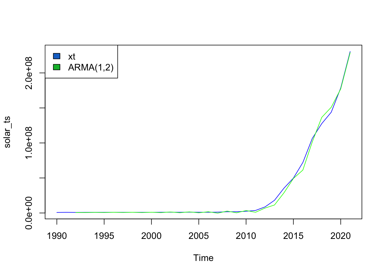
Solar
The ARMA(p,q) model that minimizes AIC is ARMA(1,2).
Call:
arma(x = solar_ts, order = c(1, 2))

Model:
ARMA(1,2)

Residuals:
     Min       1Q   Median       3Q      Max
-8923843   -53422   331446  1505395 10832340

Coefficient(s):
            Estimate  Std. Error  t value Pr(>|t|)
ar1        1.268e+00   1.864e-02   68.028  < 2e-16 ***
ma1        1.018e+00   1.741e-01    5.849 4.96e-09 ***
ma2       -2.671e-01   2.142e-01   -1.247    0.212
intercept -5.627e+05         NaN      NaN      NaN
---
Signif. codes:  0 '***' 0.001 '**' 0.01 '*' 0.05 '.' 0.1 ' ' 1

Fit:
sigma^2 estimated as 1.255e+13,  Conditional Sum-of-Squares = 3.82509e+14,  AIC = 1063.94
Simiarly, ARMA(1,2) for solar produces an AIC value of 1,063.94 and a CSS value of 3.82x10^9. The model fits this data much better than the previous data as it follows a steadier upward trend over time as solar production has been more widely adopted by US states. Additionally, solar power is less prone to political shocks so is easier to predict and fit.
\[ \phi(B) = 1 - 1.268(B) \] \[ \theta(B) = 1 - 1.018(B) + 2.671*10^-1*(B^2) \]
5) Fit an ARMA(p,q) model using auto.arima()
Coal
Series: coal_ts
ARIMA(2,2,2)

Coefficients:
          ar1      ar2      ma1     ma2
      -0.2910  -0.8112  -0.7750  0.8498
s.e.   0.1896   0.1227   0.2165  0.3065

sigma^2 = 2.109e+16:  log likelihood = -606.73
AIC=1223.45   AICc=1225.95   BIC=1230.46
Auto.arima() chooses AR(2,2) as the best model, very different from my chosen model of AR(1,3). This is likely because auto.arima() considers a more comprehensive set of parameters (i.e. I didn’t check p=2 as a possible value) and I chose my model based on AIC alone whereas auto.arima() chooses models based on AIC, BIC, and AICc.
Nuclear
Series: nuclear_ts
ARIMA(0,1,0) with drift

Coefficients:
         drift
      12988794
s.e.   7504730

sigma^2 = 1.79e+15:  log likelihood = -587.85
AIC=1179.71   AICc=1180.13   BIC=1182.57
The model chosen here is (0,1,0) which is bizarre. This only applies differencing, but doesn’t use AutoRegressive modeling or Moving Average modeling. This is likely because the data is hard to fit.
Wind
Series: wind_ts
ARIMA(0,2,1)

Coefficients:
          ma1
      -0.4339
s.e.   0.1699

sigma^2 = 2.172e+14:  log likelihood = -537.34
AIC=1078.68   AICc=1079.13   BIC=1081.49
The model chosen is ARIMA(0,2,1), which is essentially an MA() model with differencing. The search algorithm decided to difference twice, where I didn’t because I already saw weak stationarity in initial exploration.
Solar
Series: solar_ts
ARIMA(0,2,1)

Coefficients:
         ma1
      0.8289
s.e.  0.1120

sigma^2 = 2.766e+13:  log likelihood = -506.9
AIC=1017.81   AICc=1018.25   BIC=1020.61
The model chosen is ARIMA(0,2,1), which is essentially an MA() model with differencing. The search algorithm decided to difference twice, where I didn’t because I already saw weak stationarity in initial exploration.
6) Forecast
Forecast each energy source for the next three years - using manually selected models, but including 2 orders of differencing for each.
Coal
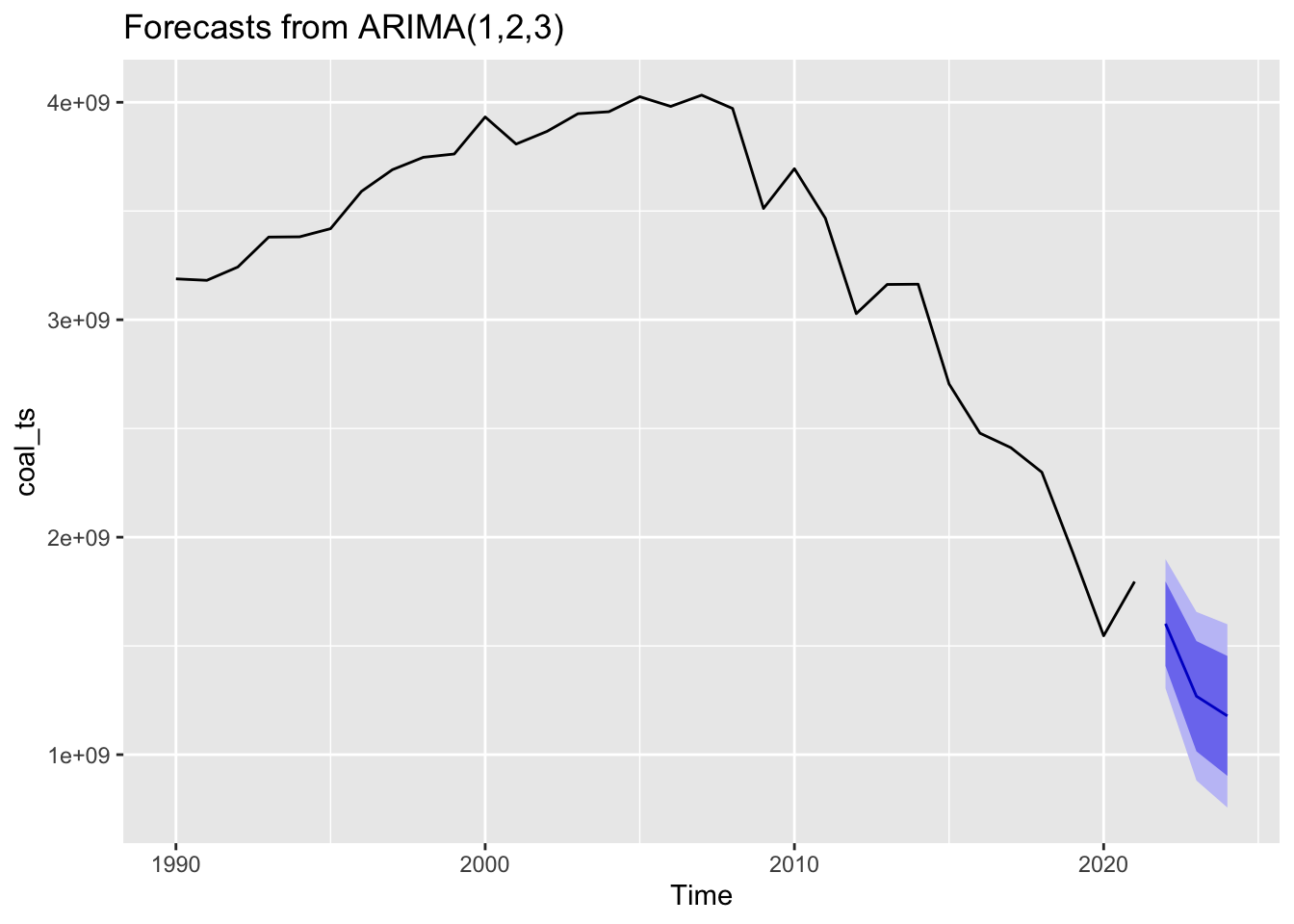
Forecasting coal production three years into the future, it’s expected to continue declining along the lines of its current downward trend. There’s quite a large confidence band around this estimate, as many other factors will affect coal production - such as the geopolitical climate surrounding coal.
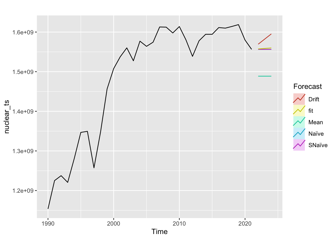
Nuclear
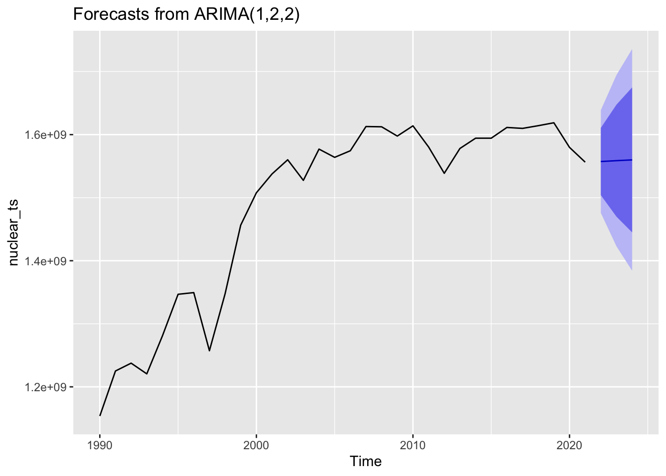
Forecasting nuclear production three years into the future, it’s expected to stay fairly steady along the 1.5x10^9 tons line. There’s quite a large confidence band around this estimate, as many other factors will affect wind production - especially political sentiment around its usage.
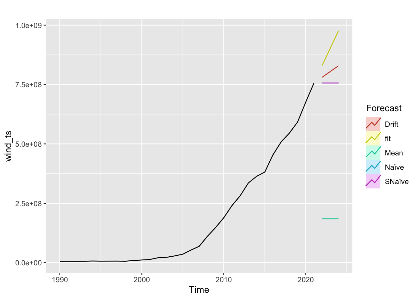
Wind
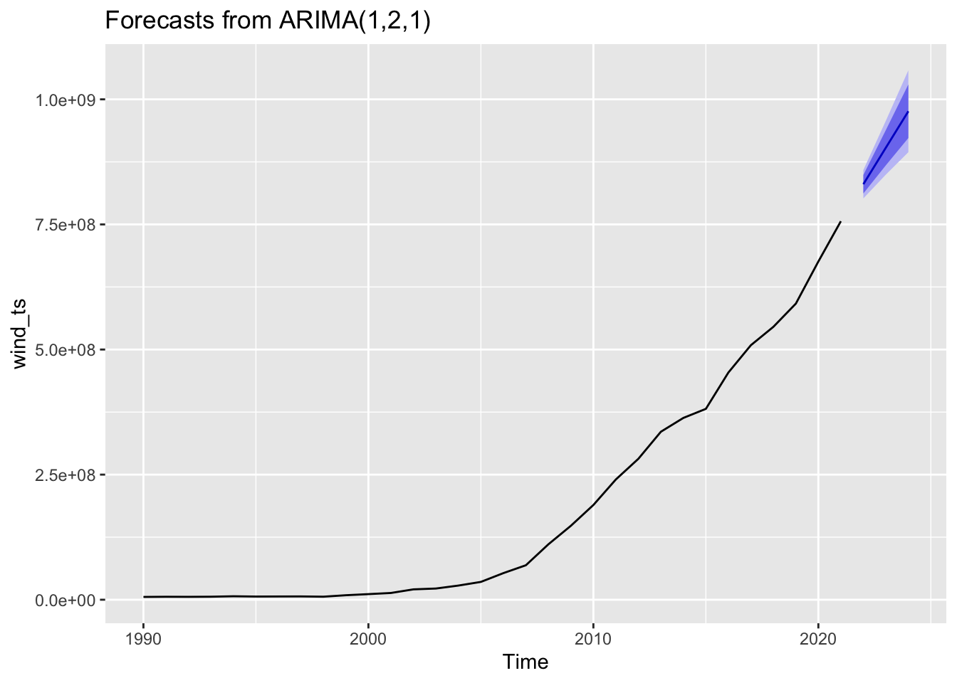
Forecasting wind production three years into the future, it’s expected to continually exponentially growing as per its existing trend. There’s a much smaller confidence band around this esimate, as its seen a steady increase over this timeframe. Infrastructure improvements in the space will affect the estimate greatly.
Solar
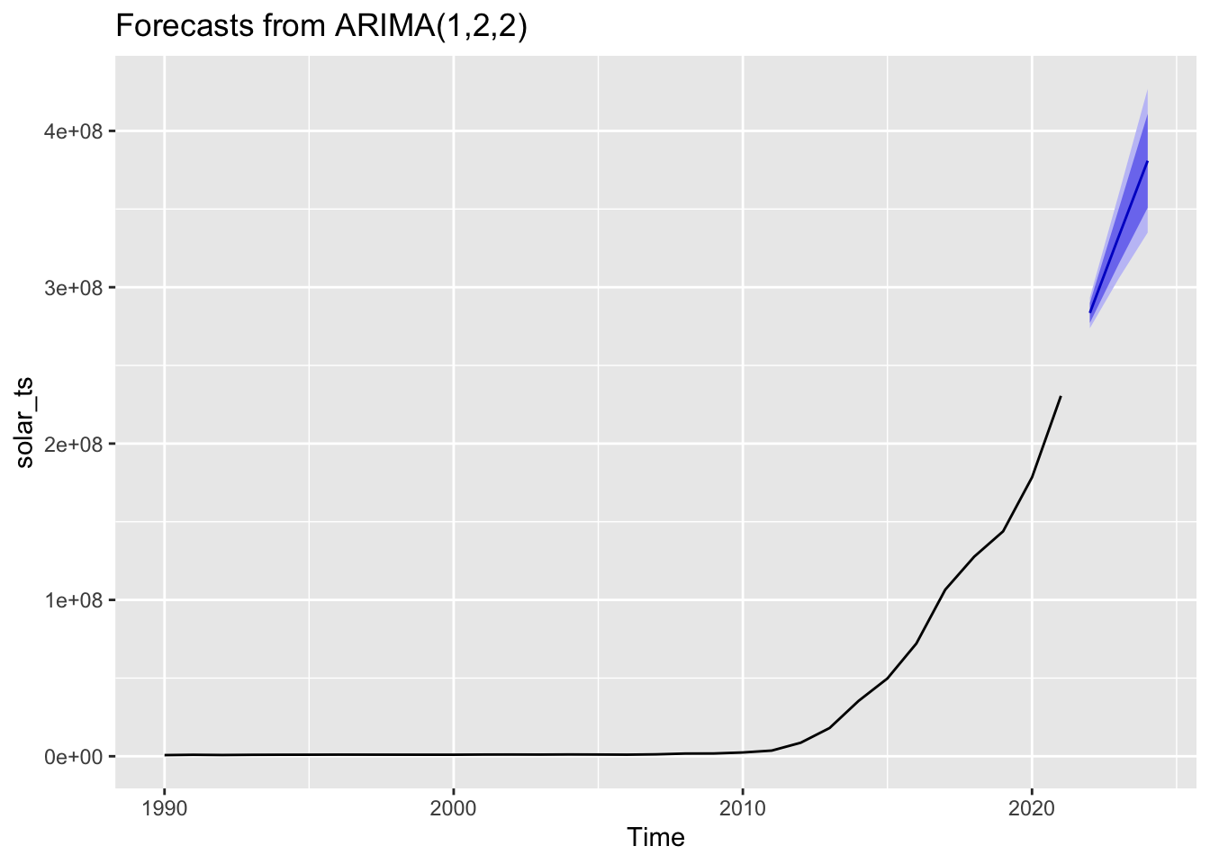
Forecasting solar production three years into the future, it’s expected to continually exponentially growing as per its existing trend. There’s a much smaller confidence band around this esimate, as its seen a steady increase over this timeframe. Infrastructure improvements in the space will affect the estimate greatly.
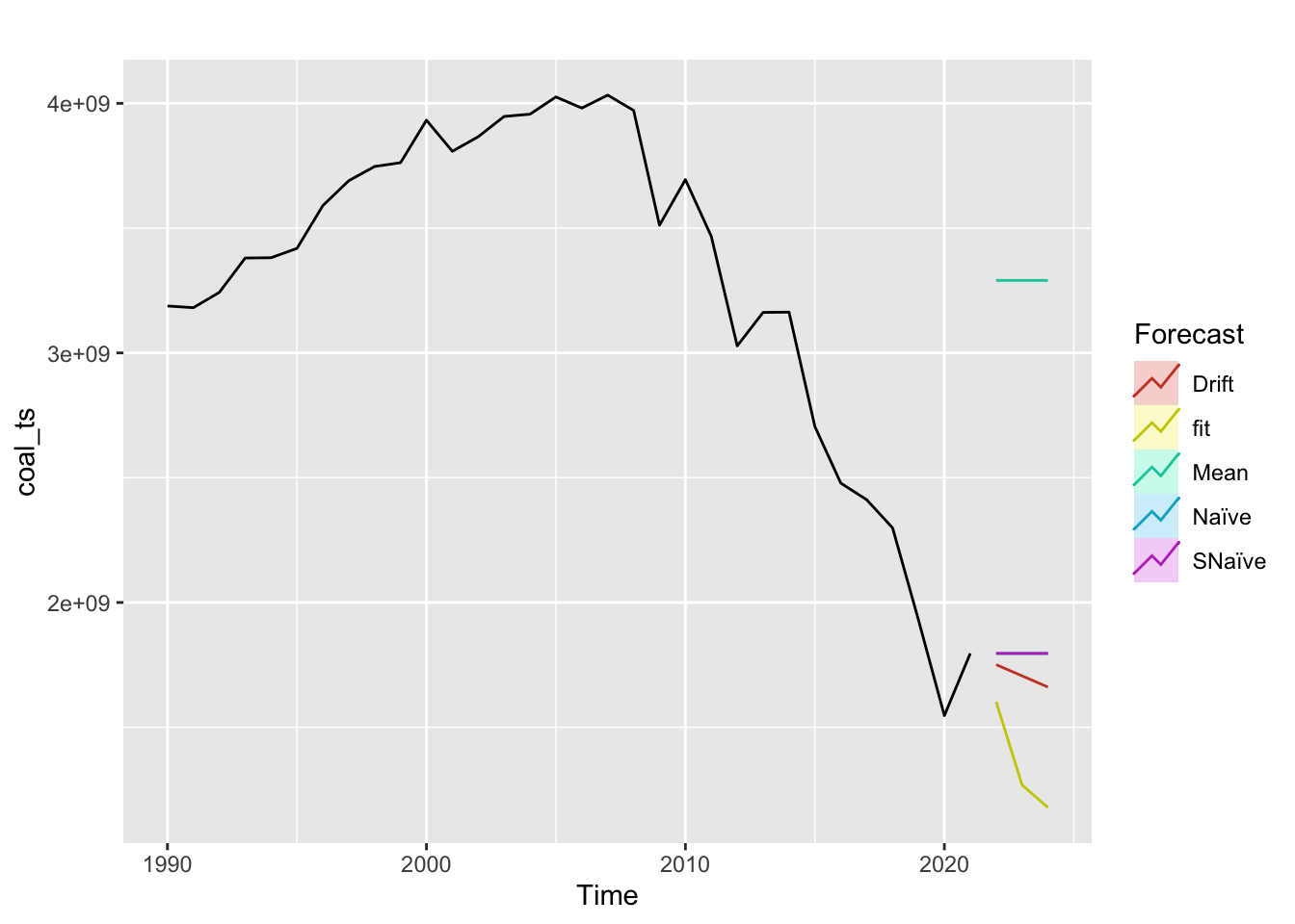
7) Benchmark Methods
Compare the models to baseline benchmark methods to ensure they’re performing above.
Coal
Nuclear
Wind
Solar
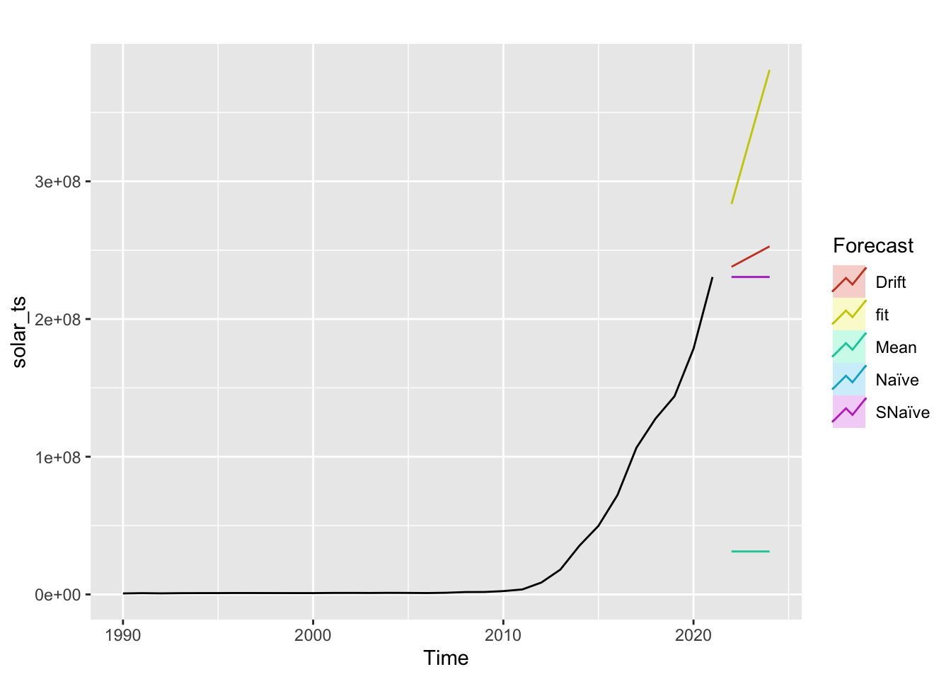
Note: Across all four energy sources, the fitted model does perform better than benchmark methods.
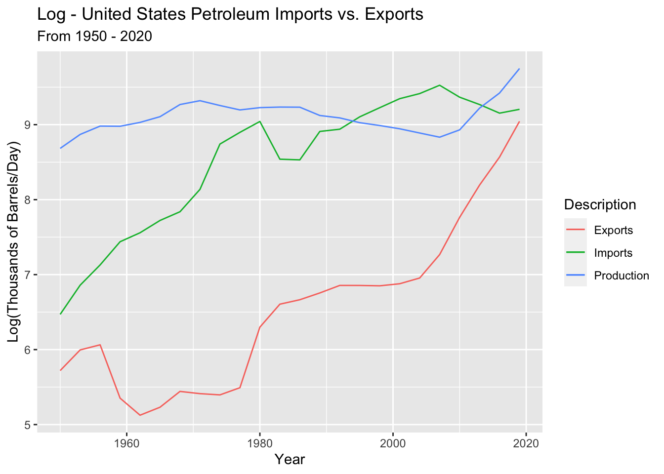
Dataset 2 - Petroleum Exports vs. Imports
1) Data Review
From EDA, we looked at ACF graphs and checked ADF to see if the data was stationary. The data was not stationary so we take the log and difference to make it stationary.
Log Transform petroleum imports, exports, and production - and plot
Since the data is still not stationary, exports, imports, and production will be differenced.
Imports
Augmented Dickey-Fuller Test
data: import_ts %>% diff()
Dickey-Fuller = -3.7192, Lag order = 2, p-value = 0.04149
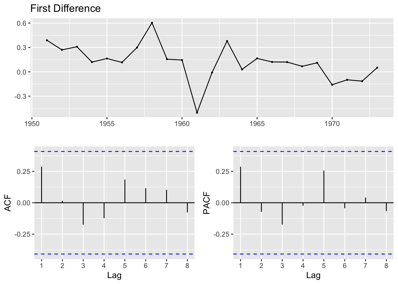
alternative hypothesis: stationaryExports
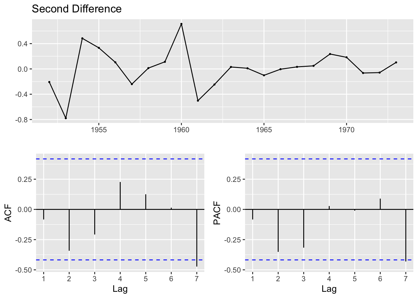
Must be differenced twice. A first difference results in a p-value of 0.32 by the ADF test: indicating that we can’t reject the null hypothesis of no stationarity. Stationarity is only achieved with a second difference.
Augmented Dickey-Fuller Test
data: export_ts %>% diff() %>% diff()
Dickey-Fuller = -4.5144, Lag order = 2, p-value = 0.01
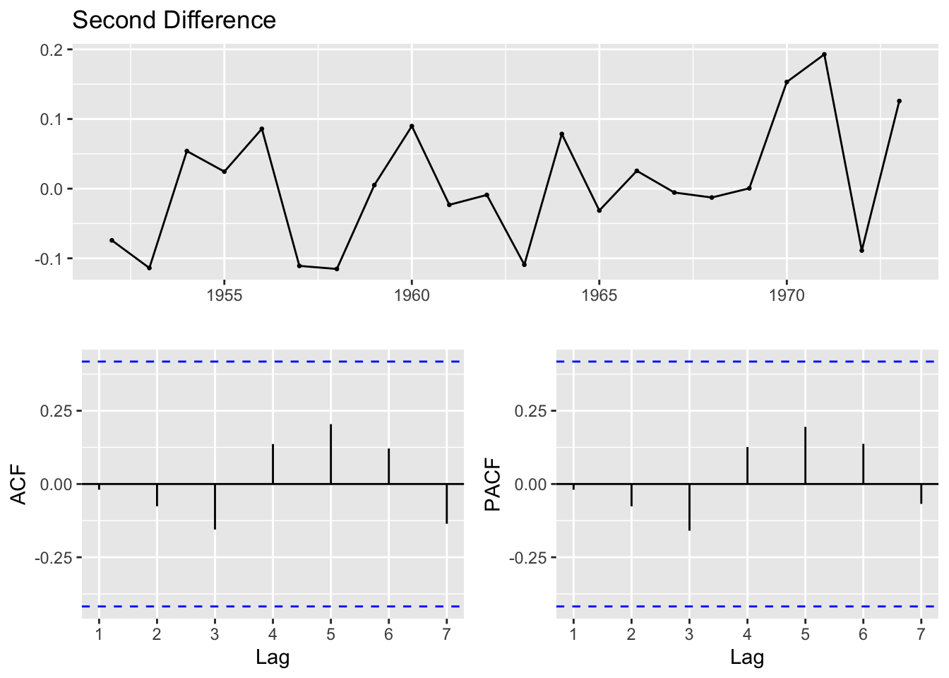
alternative hypothesis: stationaryProduction Must be differenced twice. A first difference results in a p-value of 0.99 by the ADF test: indicating that we can’t reject the null hypothesis of no stationarity. Stationarity is only achieved with a second difference.
    Augmented Dickey-Fuller Test

data:  production_ts %>% diff() %>% diff()
Dickey-Fuller = -4.0549, Lag order = 2, p-value = 0.02134
alternative hypothesis: stationary
All three variables were differenced once or twice in order to achieve stationarity. The stationary property of the data is confirmed by the ACF plots of each, as well as the Augmented-Dickey-Fuller Test of the differenced series.
2) ACF/PACF Plots
ACF/PACF plots are used to select potential p and q values for an ARIMA(p,d,q) model. From these plots, some potential p and q values are selected to fit an ARIMA model with. Separate models have to be fit for each variable thus separate ACF/PACF plots are shown below.
Import
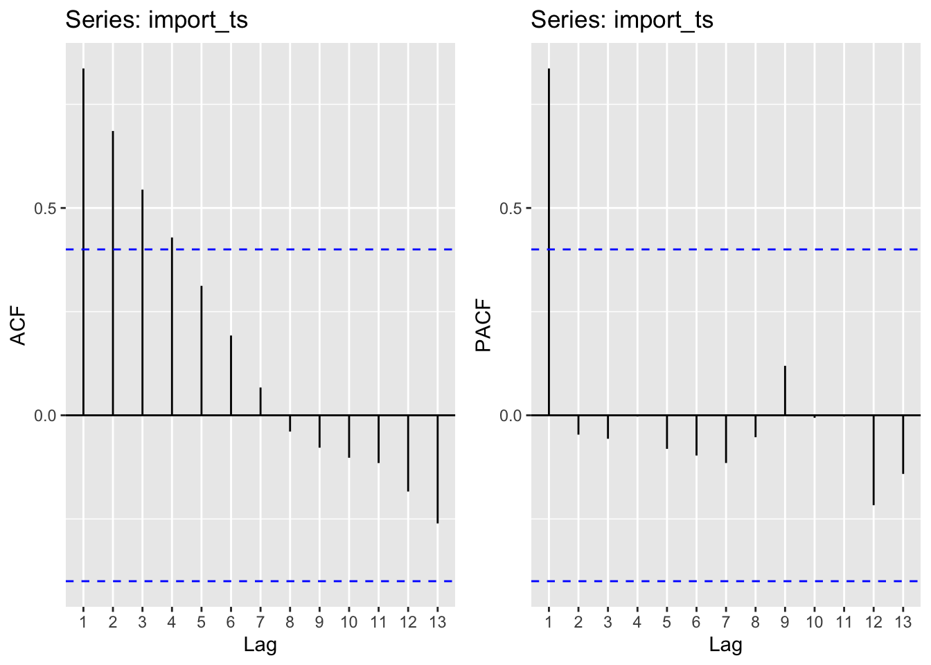
Moving average order (found from ACF): q - 1,2,3
Autoregressive term (found from pACF): p - 1
Exports
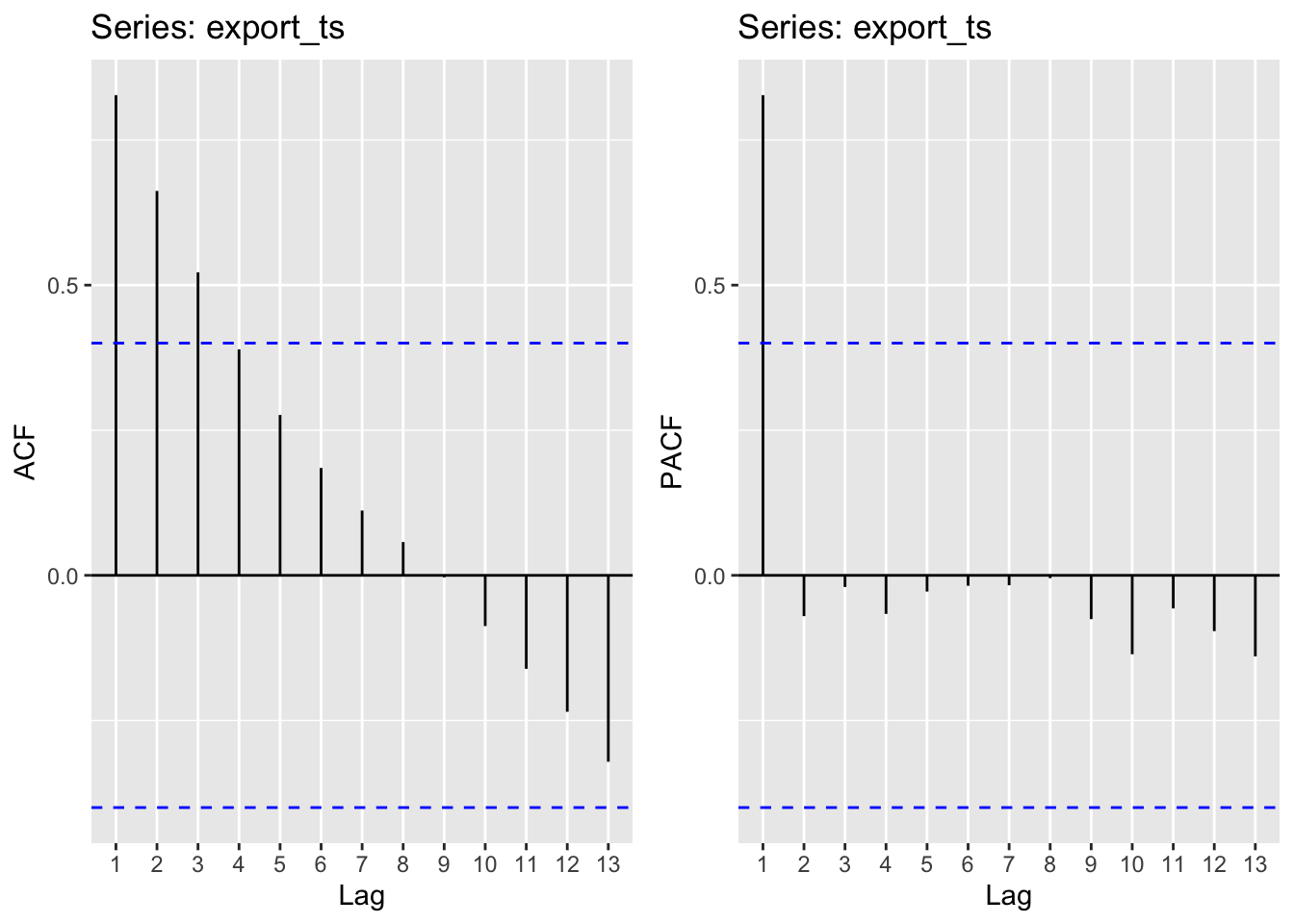
Moving average order (found from ACF): q - 1,2,3
Autoregressive term (found from pACF): p - 1
Production
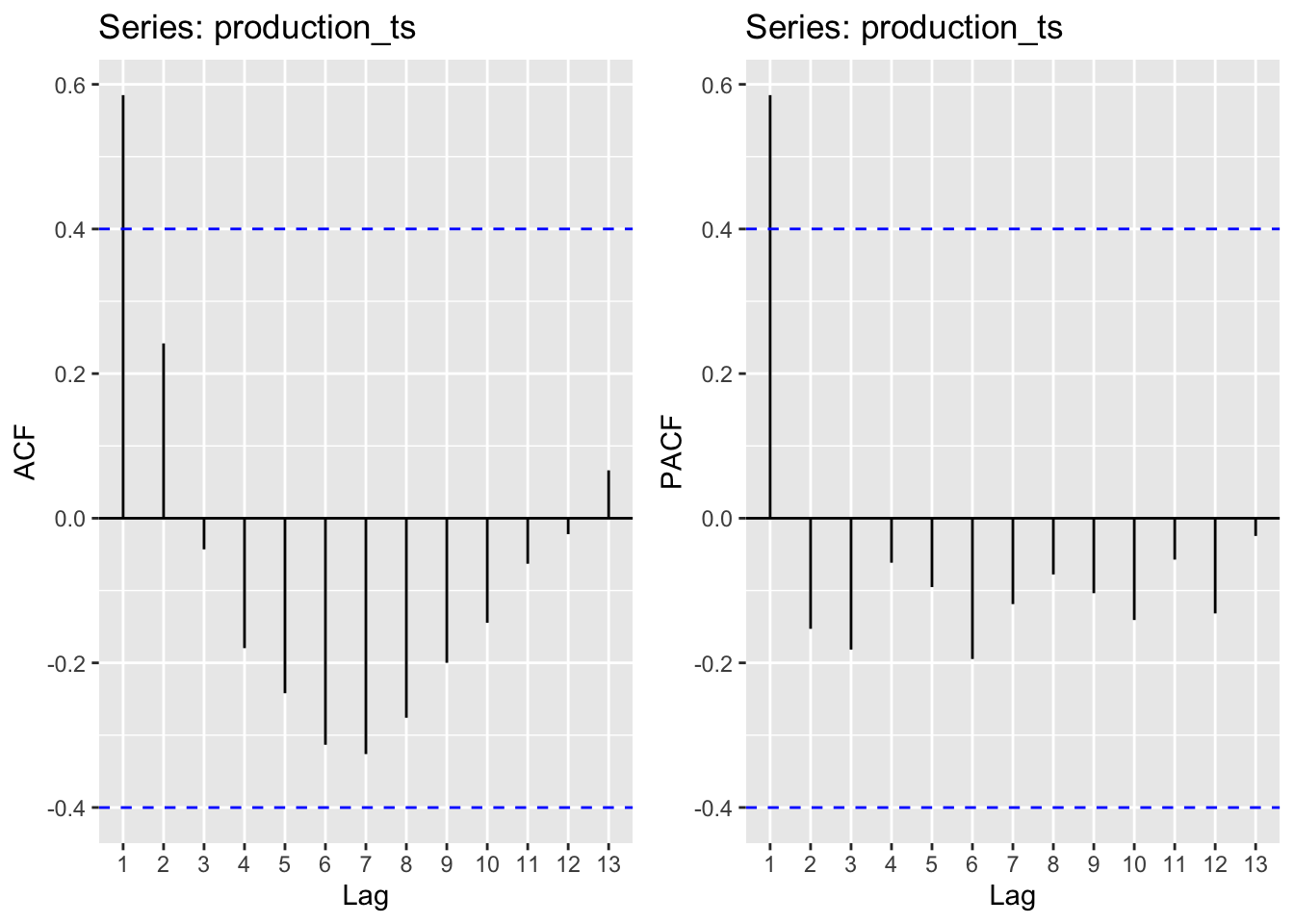
Moving average order (found from ACF): q - 1
Autoregressive term (found from pACF): p - 1
3) Fit ARIMA(p,d,q) models
Imports
| p | d | q | AIC | BIC | AICc |
|---|---|---|---|---|---|
| 1 | 1 | 1 | 1.764891 | 5.171374 | 3.028049 |
| 1 | 2 | 1 | 1.782784 | 5.055911 | 3.116117 |
| 1 | 3 | 1 | 10.774584 | 13.908151 | 12.186349 |
| 1 | 1 | 2 | 3.519834 | 8.061811 | 5.742056 |
| 1 | 2 | 2 | 3.708435 | 8.072605 | 6.061376 |
| 1 | 3 | 2 | 7.919693 | 12.097783 | 10.419693 |
| 1 | 1 | 3 | 3.394707 | 9.072178 | 6.924119 |
| 1 | 2 | 3 | 5.588815 | 11.044027 | 9.338815 |
| 1 | 3 | 3 | 8.751611 | 13.974223 | 12.751611 |
Exports
| p | d | q | AIC | BIC | AICc |
|---|---|---|---|---|---|
| 1 | 1 | 1 | 10.408080 | 13.81456 | 11.67124 |
| 1 | 2 | 1 | 11.644777 | 14.91790 | 12.97811 |
| 1 | 3 | 1 | 19.463857 | 22.59742 | 20.87562 |
| 1 | 1 | 2 | 9.090324 | 13.63230 | 11.31255 |
| 1 | 2 | 2 | 12.512548 | 16.87672 | 14.86549 |
| 1 | 3 | 2 | 21.466731 | 25.64482 | 23.96673 |
| 1 | 1 | 3 | 11.089958 | 16.76743 | 14.61937 |
| 1 | 2 | 3 | 11.108577 | 16.56379 | 14.85858 |
| 1 | 3 | 3 | 18.917698 | 24.14031 | 22.91770 |
Production
| p | d | q | AIC | BIC | AICc |
|---|---|---|---|---|---|
| 1 | 1 | 0 | -42.47036 | -40.19937 | -41.87036 |
| 1 | 2 | 0 | -40.83047 | -38.64838 | -40.19889 |
| 1 | 3 | 0 | -29.22643 | -27.13739 | -28.55977 |
| 1 | 1 | 1 | -40.55816 | -37.15168 | -39.29500 |
| 1 | 2 | 1 | -38.89113 | -35.61800 | -37.55780 |
| 1 | 3 | 1 | -33.56462 | -30.43105 | -32.15285 |
| 2 | 1 | 0 | -40.56932 | -37.16284 | -39.30617 |
| 2 | 2 | 0 | -38.93721 | -35.66408 | -37.60387 |
| 2 | 3 | 0 | -28.70668 | -25.57311 | -27.29491 |
| 2 | 1 | 1 | -38.76965 | -34.22767 | -36.54743 |
| 2 | 2 | 1 | -37.03220 | -32.66803 | -34.67926 |
| 2 | 3 | 1 | -32.16038 | -27.98229 | -29.66038 |
4) Model Diagnostics
With the above exploration, a best fit model for each variable is chosen by minimizing AIC, AICc, and BIC
Imports
The ARIMA model that minimizes AIC and AICc is ARIMA(1,1,1)
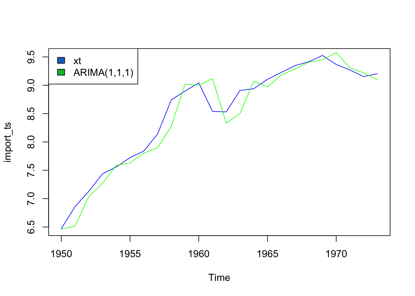
Call:
arima(x = import_ts, order = c(1, 1, 1))

Coefficients:
         ar1      ma1
      0.5586  -0.1272
s.e.  0.4354   0.5220

sigma^2 estimated as 0.04819:  log likelihood = 2.12,  aic = 1.76

Training set error measures:
                     ME      RMSE       MAE       MPE     MAPE      MASE
Training set 0.05626467 0.2149074 0.1541133 0.7196743 1.833747 0.7871504
                   ACF1
Training set -0.0981568
With this model, we get a training RMSE of 0.215, so the model fits the training data fairly well without overfitting due to its bizarre behavior.
\[ \phi(B) = 1 - 0.5586(B) \] \[ \theta(B) = 1 - 0.4354(B) \]
Exports
The consensus across AIC, BIC, and AICc is that the best fit model is ARIMA(1,1,2).
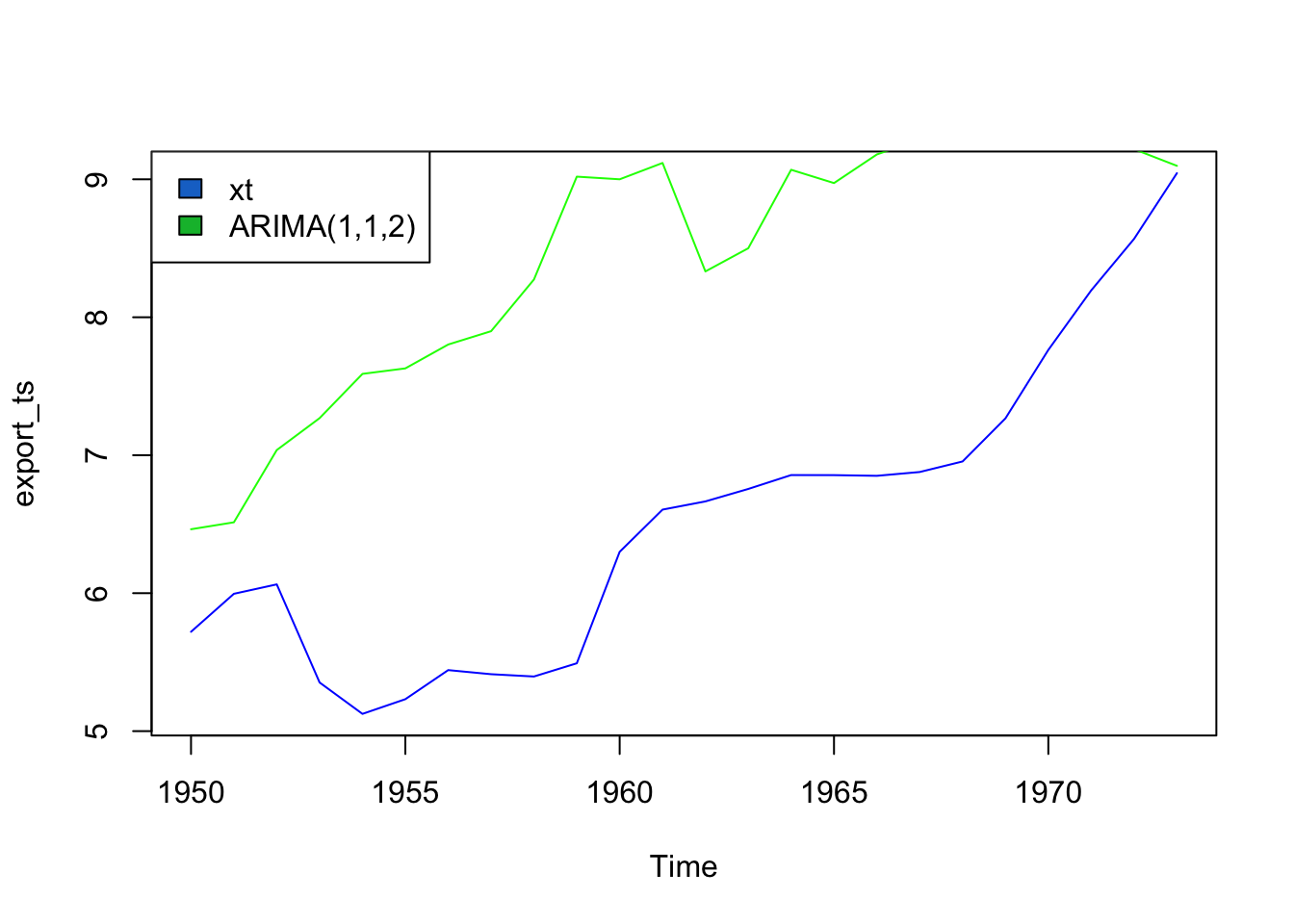
Call:
arima(x = export_ts, order = c(1, 1, 2))

Coefficients:
          ar1     ma1     ma2
      -0.8486  1.7381  0.9117
s.e.   0.1701  0.3518  0.3438

sigma^2 estimated as 0.05395:  log likelihood = -0.55,  aic = 9.09

Training set error measures:
                     ME      RMSE       MAE       MPE     MAPE      MASE
Training set 0.07329069 0.2273772 0.1747664 0.9874671 2.719147 0.7576492
                   ACF1
Training set -0.0979957
\[ \phi(B) = 1 + 0.8486(B) \] \[ \theta(B) = 1 - 1.7101(B) - 0.9117(B^2) \] With this model, we get a training RMSE of 0.2273. As evidenced by the plot, the model does a pretty terrible job with this model fit - likely due to the complex adn random nature of the data. Let’s see what auto.arima() would have chosen for this model.
Production
The consensus across AIC, BIC, and AICc is that the best fit model is ARIMA(1,1,0).
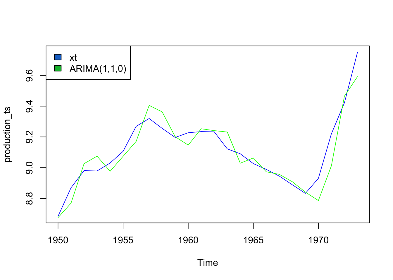
Call:
arima(x = production_ts, order = c(1, 1, 0))

Coefficients:
         ar1
      0.8427
s.e.  0.1421

sigma^2 estimated as 0.007357:  log likelihood = 23.24,  aic = -42.47

Training set error measures:
                     ME       RMSE        MAE       MPE     MAPE      MASE
Training set 0.01526092 0.08398331 0.06473024 0.1645849 0.705565 0.7023005
                    ACF1
Training set 0.008829977
\[ \phi(B) = 1 - 0.8427(B) \]
With this model, we get a training RMSE of 0.08398331, so the model fits the training data fairly well without overfitting due to its bizarre behavior.
5) Fit an ARIMA(p,d,q) model using auto.arima()
Imports
Series: import_ts
ARIMA(0,1,0) with drift

Coefficients:
       drift
      0.1189
s.e.  0.0450

sigma^2 = 0.04869:  log likelihood = 2.63
AIC=-1.26   AICc=-0.66   BIC=1.01
The model chosen is ARIMA(0,1,0) with drift. While auto.arima() agrees with my choice of differencing, it chose different parameters for p and q, and experimented with drift whereas I did not.
Exports
Series: export_ts
ARIMA(0,1,1) with drift

Coefficients:
         ma1   drift
      0.4822  0.1498
s.e.  0.1514  0.0766

sigma^2 = 0.06913:  log likelihood = -1
AIC=7.99   AICc=9.26   BIC=11.4
The model chosen is ARIMA(0,1,1) with drift. This is slightly different than my choice, likely because auto.arima() experimented with a wider range of parameters and experimented with drift.
Production
Series: production_ts
ARIMA(2,0,0) with non-zero mean

Coefficients:
         ar1      ar2    mean
      1.7223  -0.8478  9.1494
s.e.  0.1344   0.1229  0.1388

sigma^2 = 0.007907:  log likelihood = 23.34
AIC=-38.69   AICc=-36.58   BIC=-33.98
The model chosen is ARIMA(2,0,0) with non-zero mean - or an AR(2) model. AR is more suitable when the data has a clear pattern of autoregression and less randomness. This potentially makes sense given the lack of seasonality and large overall upward trend in production since 1970.
6) Forecast
Forecasting petroleum imports, exports, and production for the next three years.
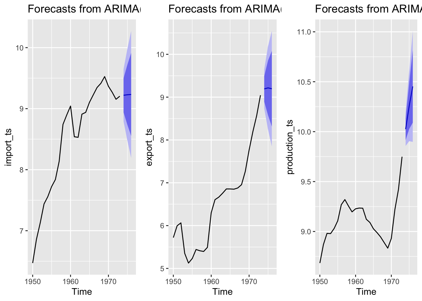
All three forecasts have a wide confidence band - indicating that based on past data alone we cannot generate a good estimate with high confidence. Imports are expected to increase slightly in the next 3 years, but have mostly stabilized. Exports are expected to increase for a year and then plateau/decrease for the next two years. Production is expected to continue exponentially increasing during the next three years.
7) Benchmark
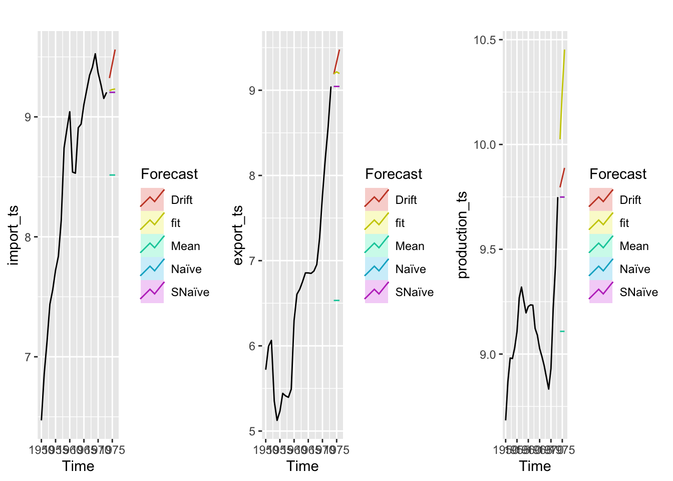
The models perform better than most of the models, expect the drift model. It’s clear that the models would benefit from incorporating a drift term to account for the intense drift especially production and exports suffer from.
Dataset 3 - Cost of Energy
1) Data Review
From EDA, we looked at ACF graphs and checked ADF to see if the data was stationary. The data was not stationary so we take the log and difference to make it stationary.
Log Transform - and plot
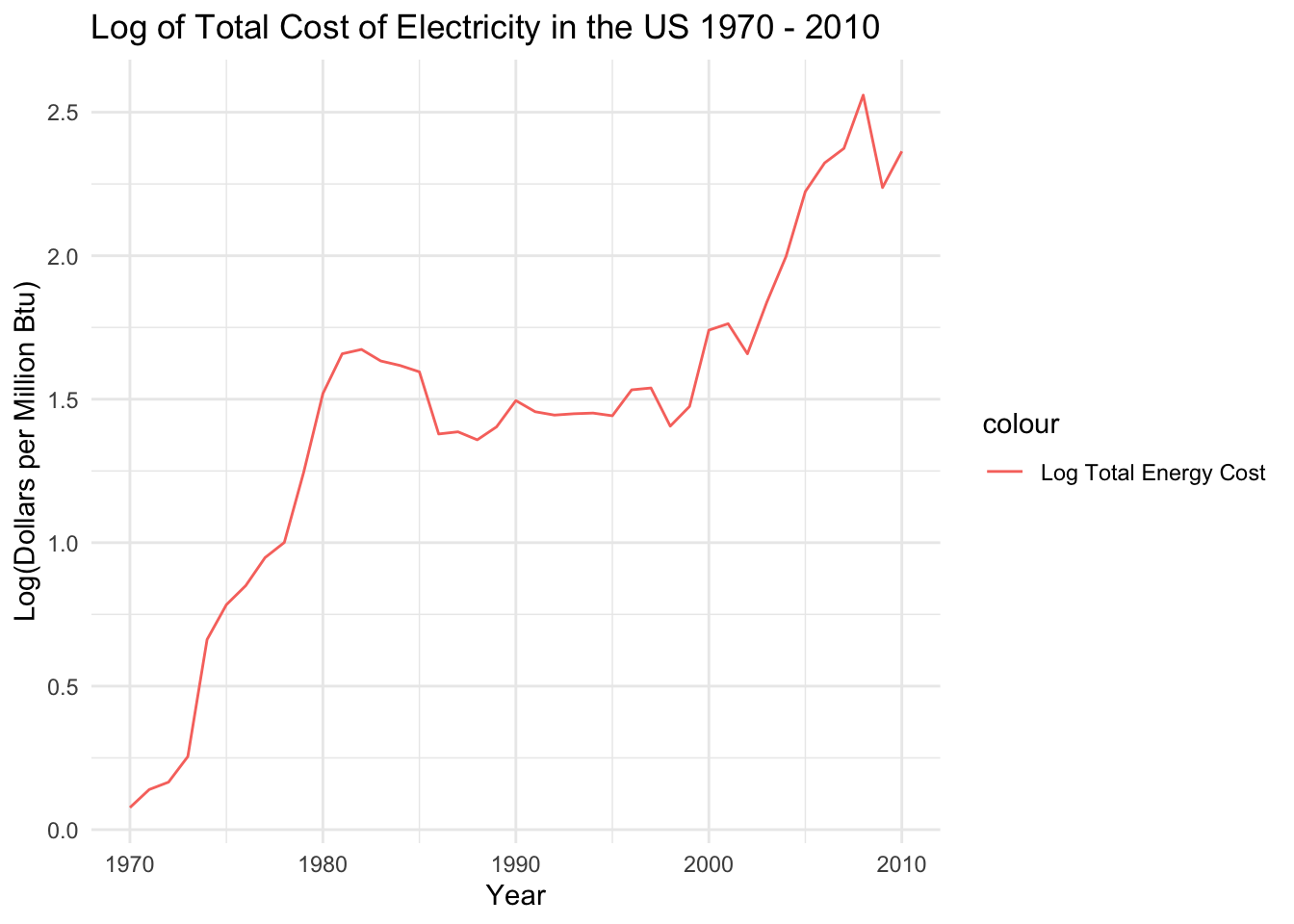
Taking the log of the data barely changed it! We’ll have to difference it. According to the ADF test, the data requires 2 differences. We can experiment with this during model building.
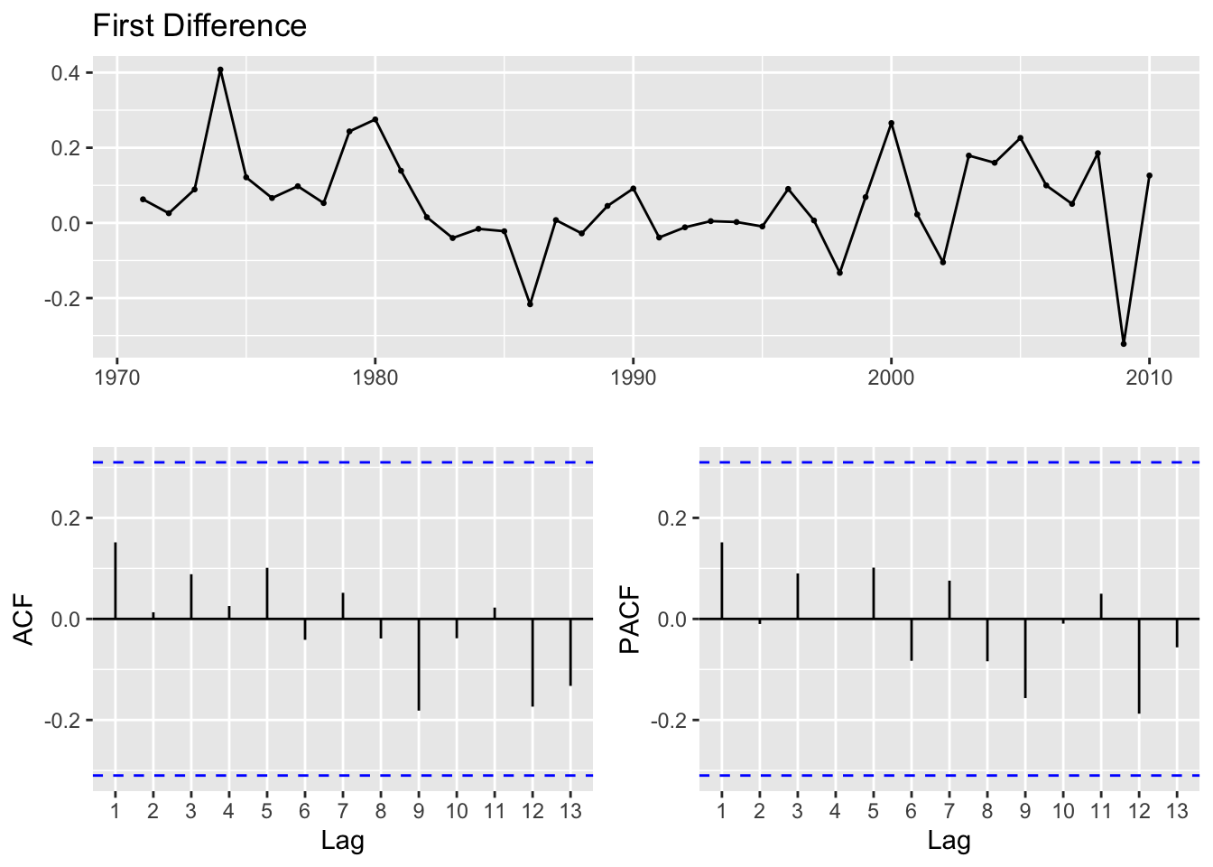
    Augmented Dickey-Fuller Test

data:  cost_ts %>% diff()
Dickey-Fuller = -2.6121, Lag order = 3, p-value = 0.3332
alternative hypothesis: stationary
2) ACF/PACF Plots
ACF/PACF plots are used to select potential p and q values for an ARIMA(p,d,q) model. From these plots, some potential p and q values are selected to fit an ARIMA model with. Separate models have to be fit for each variable thus separate ACF/PACF plots are shown below.
Import
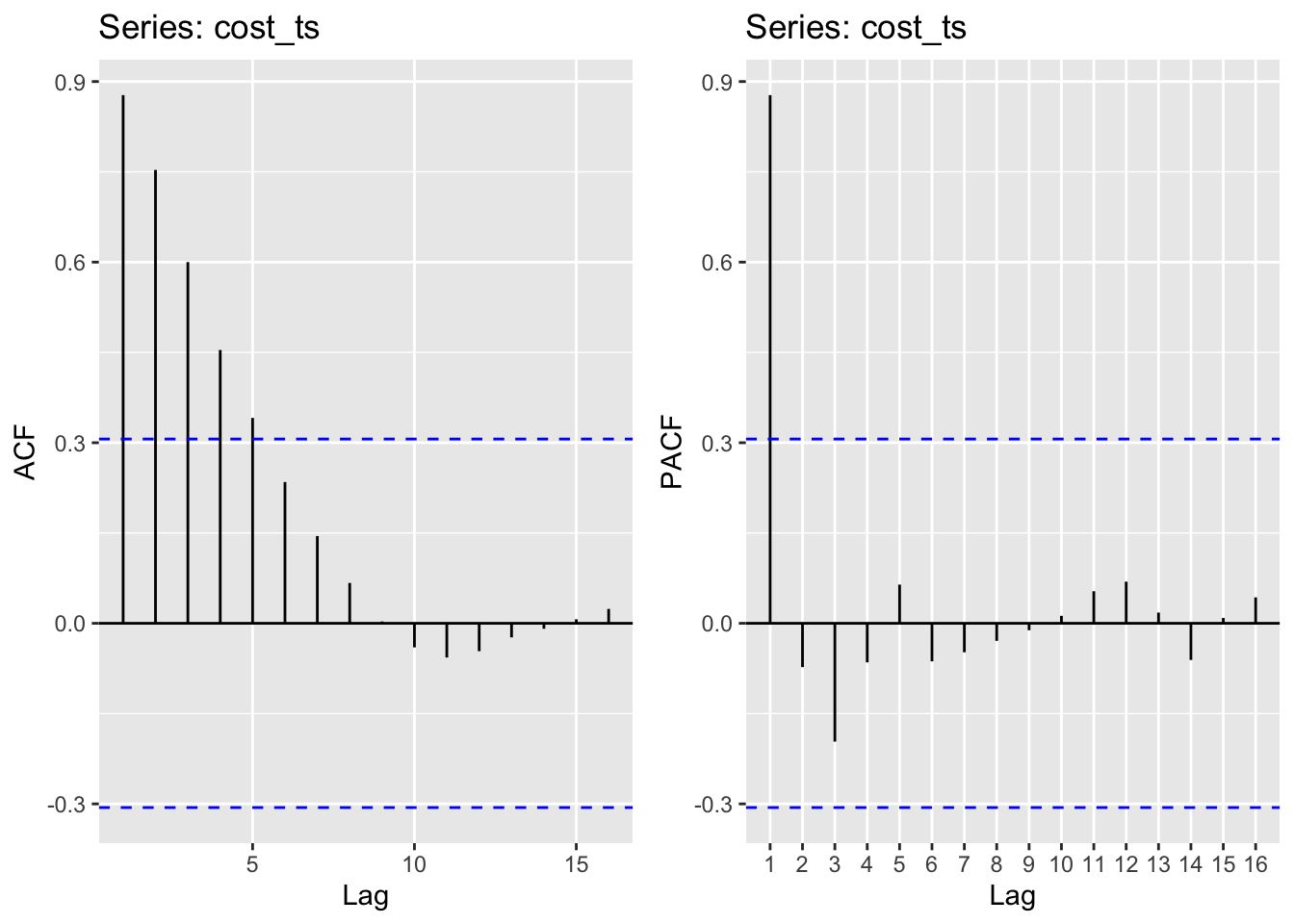
Moving average order (found from ACF): q - 1,2,3,4,5
Autoregressive term (found from pACF): p - 0,1
3) Fit ARIMA(p,d,q) models
| p | d | q | AIC | BIC | AICc |
|---|---|---|---|---|---|
| 0 | 2 | 1 | -39.93109 | -36.60397 | -39.59776 |
| 0 | 3 | 1 | -17.18553 | -13.91036 | -16.84267 |
| 0 | 2 | 2 | -38.52660 | -33.53591 | -37.84088 |
| 0 | 3 | 2 | -29.18752 | -24.27477 | -28.48164 |
| 0 | 2 | 3 | -36.60530 | -29.95105 | -35.42883 |
| 0 | 3 | 3 | -27.35465 | -20.80430 | -26.14253 |
| 0 | 2 | 4 | -37.89350 | -29.57569 | -36.07532 |
| 0 | 3 | 4 | -26.43893 | -18.25100 | -24.56393 |
| 0 | 2 | 5 | -36.23746 | -26.25609 | -33.61246 |
| 0 | 3 | 5 | -26.28811 | -16.46259 | -23.57843 |
| 1 | 2 | 1 | -38.52145 | -33.53077 | -37.83574 |
| 1 | 3 | 1 | -22.09809 | -17.18533 | -21.39221 |
| 1 | 2 | 2 | -39.77465 | -33.12040 | -38.59818 |
| 1 | 3 | 2 | -27.31762 | -20.76727 | -26.10550 |
| 1 | 2 | 3 | -37.90967 | -29.59186 | -36.09149 |
| 1 | 3 | 3 | -28.53833 | -20.35040 | -26.66333 |
| 1 | 2 | 4 | -36.48416 | -26.50279 | -33.85916 |
| 1 | 3 | 4 | -27.12777 | -17.30225 | -24.41809 |
| 1 | 2 | 5 | -34.48427 | -22.83934 | -30.87137 |
| 1 | 3 | 5 | -25.13525 | -13.67215 | -21.40192 |
4) Model Diagnostics
With the above exploration, a best fit model for each variable is chosen by minimizing AIC, AICc, and BIC
The ARIMA model that minimizes AIC, BIC, and AICc is ARIMA(0,2,1)
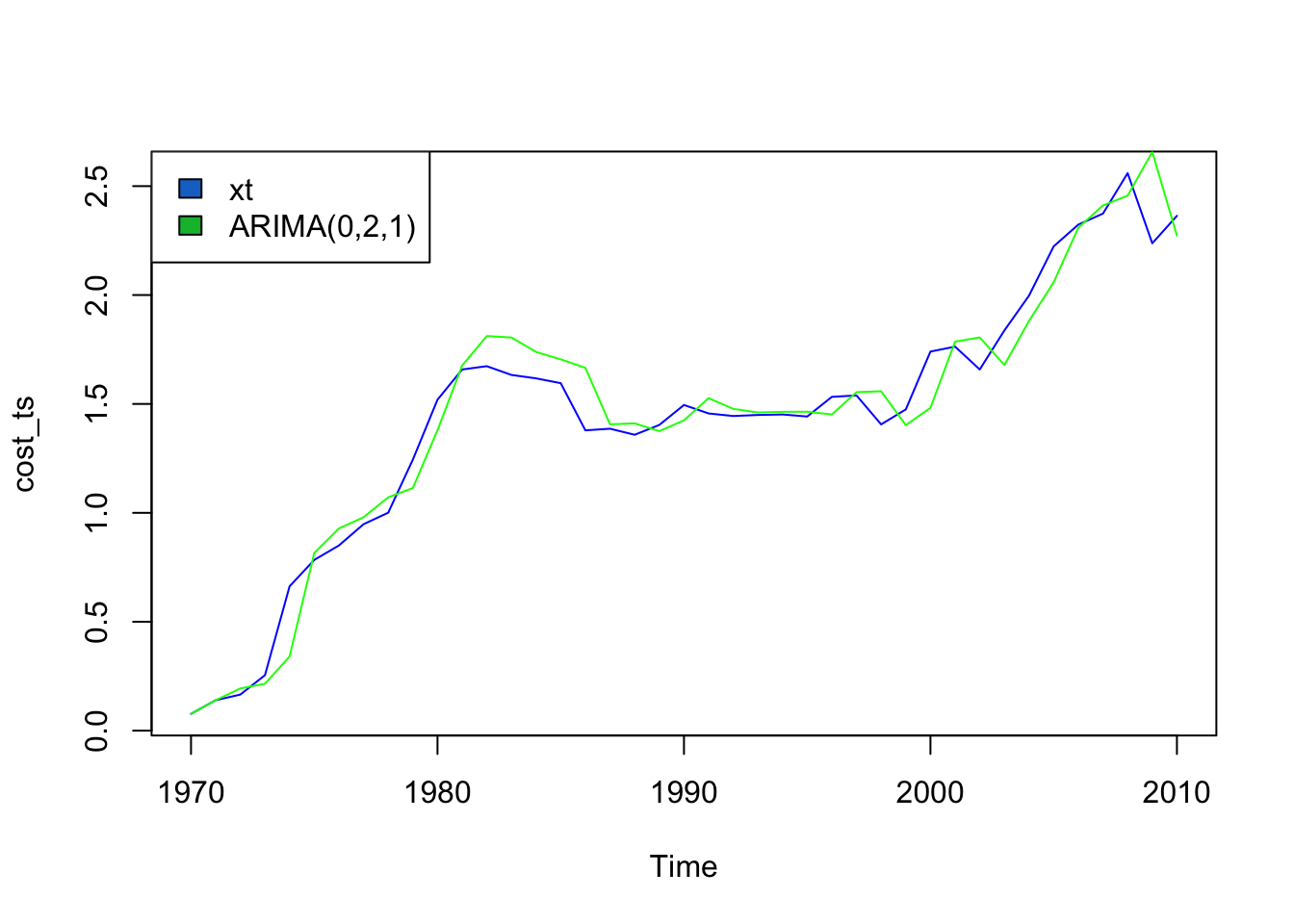
Call:
arima(x = cost_ts, order = c(0, 2, 1))

Coefficients:
          ma1
      -0.8515
s.e.   0.1333

sigma^2 estimated as 0.01836:  log likelihood = 21.97,  aic = -39.93

Training set error measures:
                       ME      RMSE        MAE        MPE     MAPE      MASE
Training set -0.007565158 0.1321637 0.09492191 -0.1831388 7.305725 0.9102723
                   ACF1
Training set 0.06219478
With this model, we get a training RMSE of 0.243, so the model fits the training data fairly well without overfitting. The random bumps and dips in the data have been largely smoothed, while the trend line is maintained.
\[ \theta(B) = 1 + 0.8616(B) \]
5) Fit an ARIMA(p,d,q) model using auto.arima()
Series: cost_ts
ARIMA(0,1,0) with drift

Coefficients:
       drift
      0.0572
s.e.  0.0207

sigma^2 = 0.01756:  log likelihood = 24.6
AIC=-45.19   AICc=-44.87   BIC=-41.81
The model chosen by auto.arima() is ARIMA(0,1,0) with drift. This is similar to the model parameters that I manually chose - except that auto.arima() chose to perform a second difference of the data and didn’t see the need for a moving average term.
6) Forecast
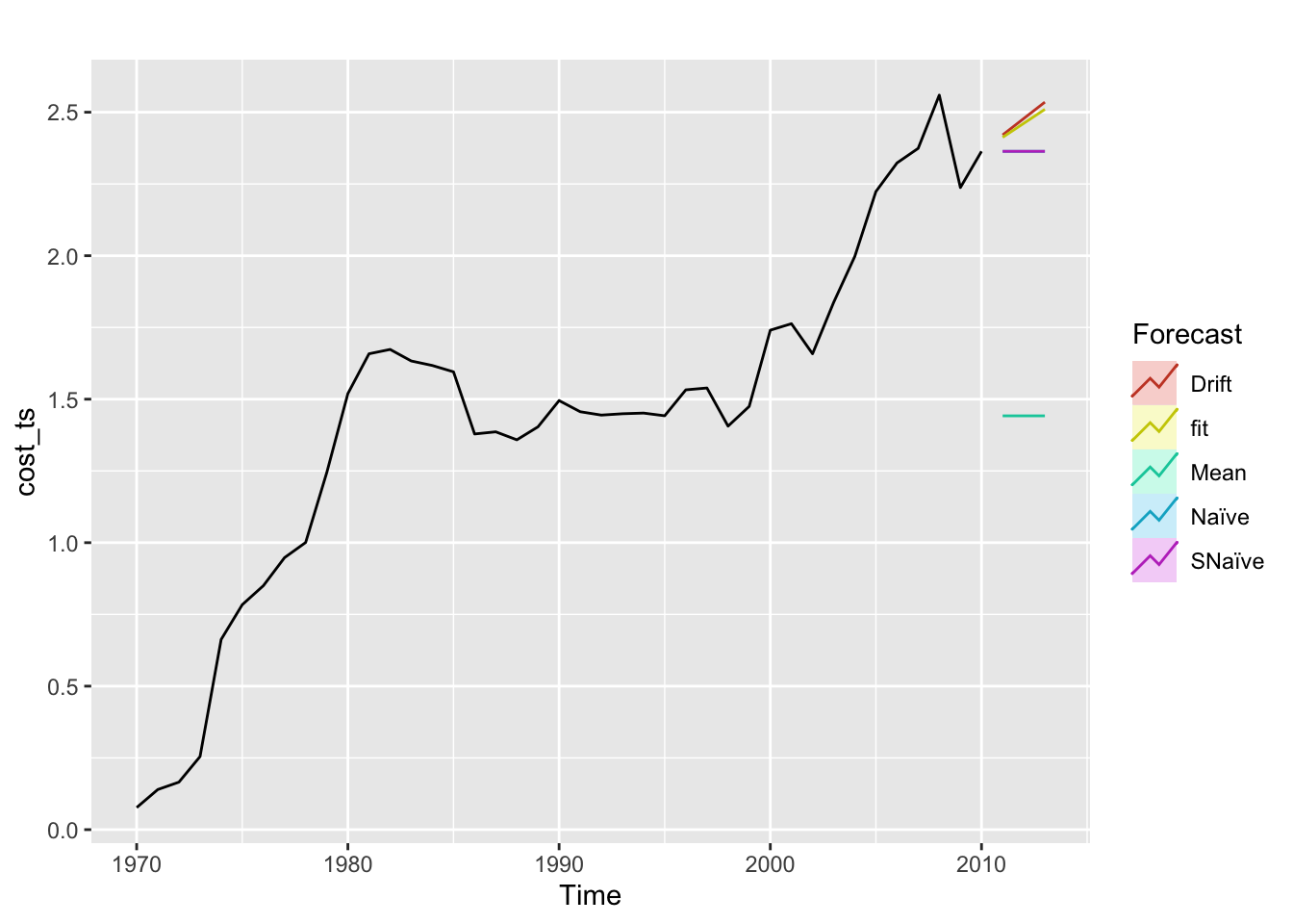
Forecasting electricity costs for the next three years.
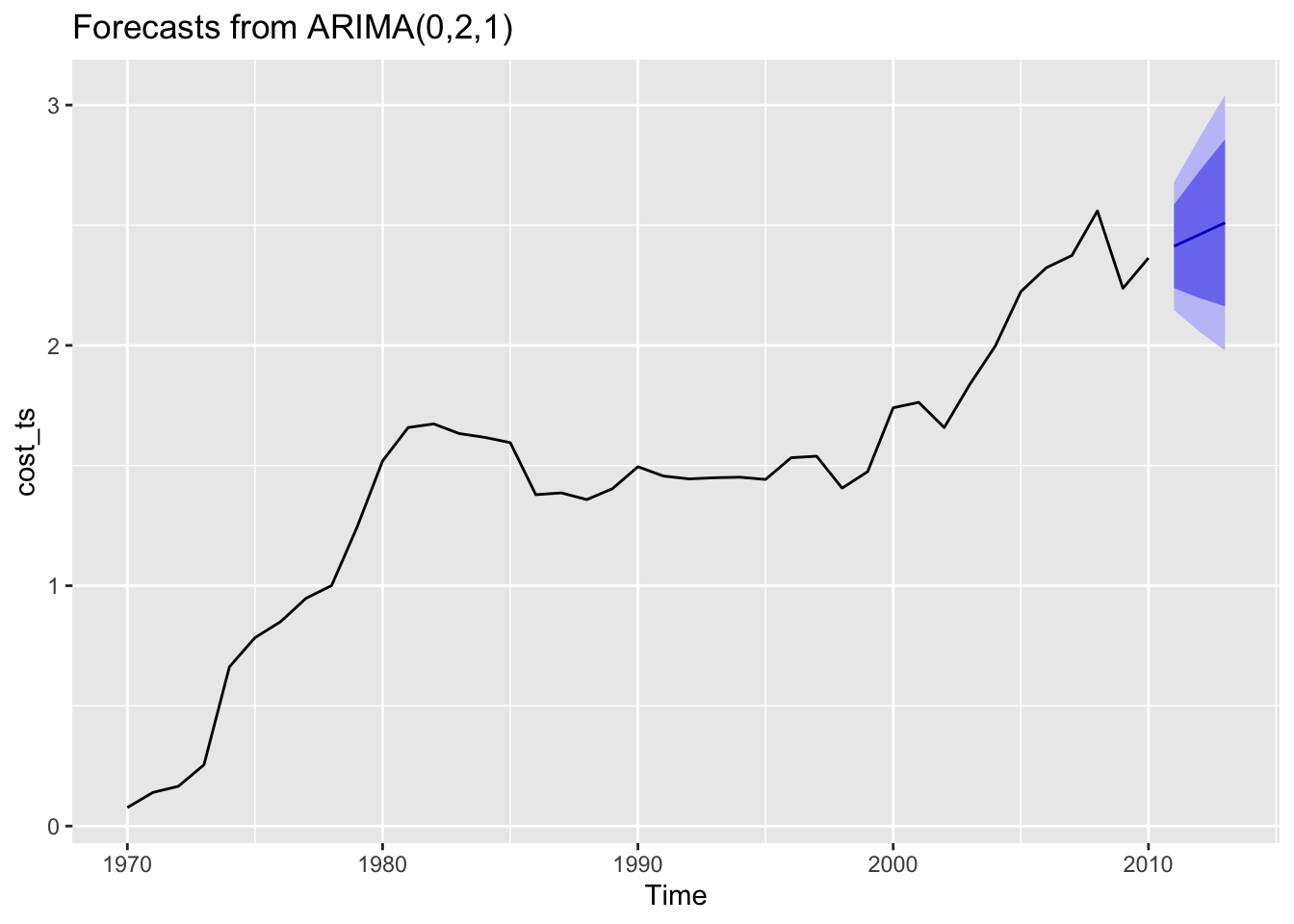
According to our model, electricity costs are going to continue to rise over the next three years. Though there is ia decently large confidence band around the estimate, it is predicted that the slight dip in electricity costs during the Great Recession in 2008 were short lived and the market is going to recover. Since this data is old, I can confirm that electricity costs have continued to rise since the dataset stopped collecting data and the model forecast was correct.
7) Benchmark
The model performs better than all the benchmark methods - except drift which performs about the same as the model. Again, this model could be improved by including a drift term and then should outperform even the drift benchmark.
Dataset 4 - CO2 Emissions
1) Data Review
From EDA, we looked at ACF graphs and checked ADF to see if the data was stationary. The data was not stationary so we take the log and difference to make it stationary.
Log Transform coal, natural gas, petro, and hydrocarbon gas - and plot
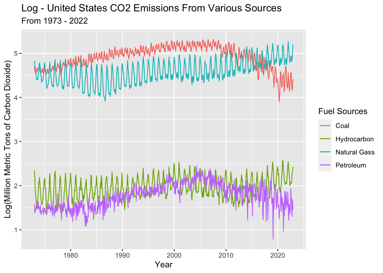
Taking the log of the data changed it significantly! An ADF test reveals the data is almost stationary. According to the ADF test, coal and petroleum require another differencing, while hydro and natural gas are already stationary. We can experiment with this during model building.
    Augmented Dickey-Fuller Test

data:  coal_ts %>% diff()
Dickey-Fuller = -17.759, Lag order = 8, p-value = 0.01
alternative hypothesis: stationary
    Augmented Dickey-Fuller Test

data:  hydro_ts
Dickey-Fuller = -4.6126, Lag order = 8, p-value = 0.01
alternative hypothesis: stationary
    Augmented Dickey-Fuller Test

data:  natural_ts
Dickey-Fuller = -5.1735, Lag order = 8, p-value = 0.01
alternative hypothesis: stationary
Augmented Dickey-Fuller Test
data: petro_ts %>% diff()
Dickey-Fuller = -14.139, Lag order = 8, p-value = 0.01
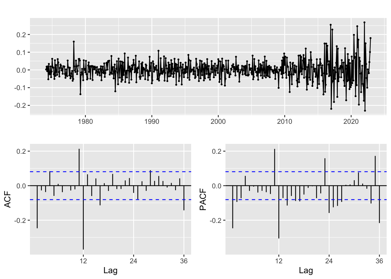
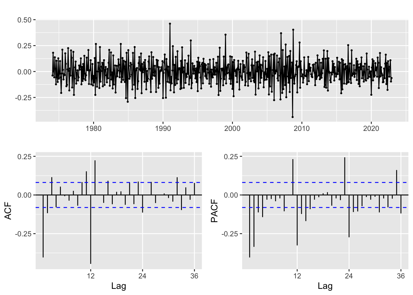
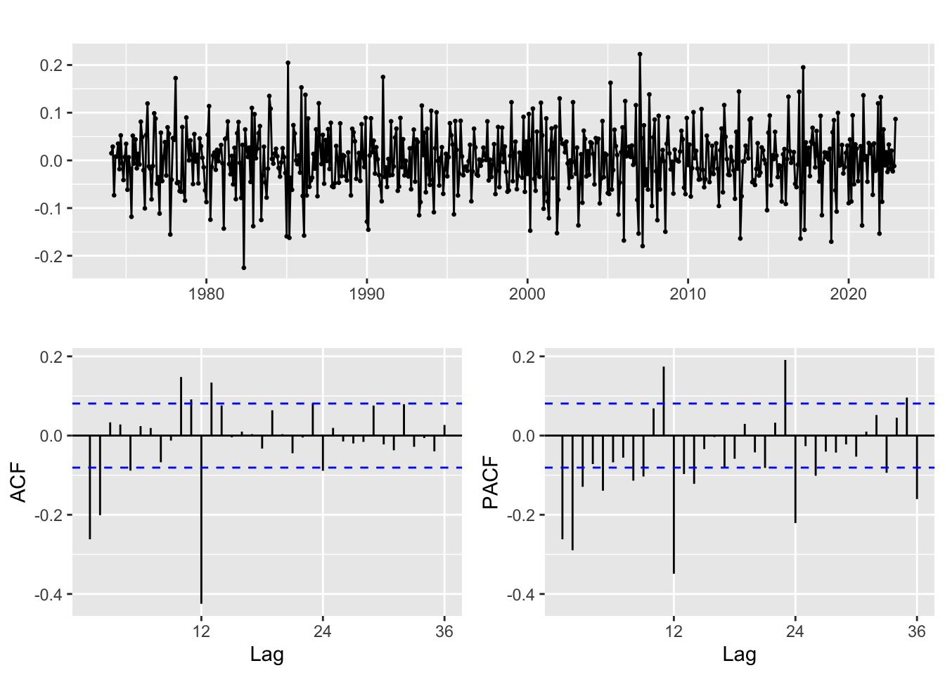
alternative hypothesis: stationary2) ACF/PACF Plots
ACF/PACF plots are used to select potential p and q values for a SARIMA(p,d,q)(P,D,Q) model. SARIMA is used because the data contains seasonal components and had differencing. From these plots, some potential p,q,P,Q values are selected to fit a SARIMA model with. Separate models have to be fit for each energy source, thus separate ACF/PACF plots are shown below.
Coal
Differencing: d = 0,1; D = 0,1
Moving average order: q = 0,1; Q = 0,1,2,3
Autoregressive terms: p = 0,1, P = 0,1
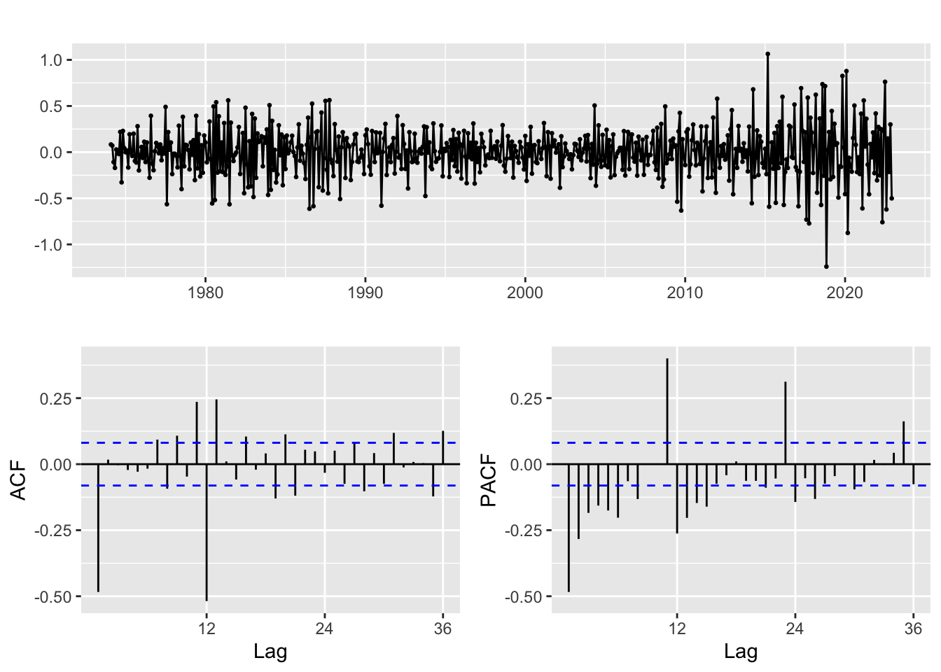
Hydrocarbon
Differencing: d = 0,1; D = 0,1
Moving average order: q = 0,1,2,3,4; Q = 0,1,2,3
Autoregressive terms: p = 0,1, P = 0,1,2
Natural Gas
Differencing: d = 0,1; D = 0,1
Moving average order (ACF): q = 0,1,2; Q = 0,1,2
Autoregressive terms (PACF): p = 0,1,2,3; P = 0,1,2,3
Petroleum
Differencing: d = 0,1; D = 0,1
Moving average order: q = 0,1; Q = 0,1
Autoregressive terms: p = 0,1,2,3,4; P = 0,1,2
3) Fit SARIMA models and Model Diagnostics
Coal
| p | d | q | P | D | Q | AIC | BIC | AICc |
|---|---|---|---|---|---|---|---|---|
| 0 | 1 | 0 | 0 | 1 | 0 | -1713.934 | -1709.559 | -1713.928 |
| 0 | 1 | 0 | 1 | 1 | 0 | -1808.766 | -1800.016 | -1808.746 |
| 0 | 1 | 0 | 0 | 1 | 1 | -1933.114 | -1924.364 | -1933.094 |
| 0 | 1 | 0 | 1 | 1 | 1 | -1934.556 | -1921.431 | -1934.515 |
| 0 | 1 | 0 | 0 | 1 | 2 | -1935.279 | -1922.154 | -1935.238 |
| 0 | 1 | 0 | 1 | 1 | 2 | -1933.530 | -1916.030 | -1933.461 |
| 0 | 1 | 1 | 0 | 1 | 0 | -1756.164 | -1747.414 | -1756.144 |
| 0 | 1 | 1 | 1 | 1 | 0 | -1840.869 | -1827.744 | -1840.828 |
| 0 | 1 | 1 | 0 | 1 | 1 | -1954.295 | -1941.170 | -1954.254 |
| 0 | 1 | 1 | 1 | 1 | 1 | -1957.260 | -1939.760 | -1957.191 |
| 0 | 1 | 1 | 0 | 1 | 2 | -1958.498 | -1940.998 | -1958.429 |
| 0 | 1 | 1 | 1 | 1 | 2 | -1956.844 | -1934.969 | -1956.741 |
| 1 | 1 | 0 | 0 | 1 | 0 | -1749.433 | -1740.683 | -1749.412 |
| 1 | 1 | 0 | 1 | 1 | 0 | -1832.690 | -1819.565 | -1832.649 |
| 1 | 1 | 0 | 0 | 1 | 1 | -1946.043 | -1932.918 | -1946.002 |
| 1 | 1 | 0 | 1 | 1 | 1 | -1949.070 | -1931.570 | -1949.001 |
| 1 | 1 | 0 | 0 | 1 | 2 | -1950.206 | -1932.706 | -1950.138 |
| 1 | 1 | 0 | 1 | 1 | 2 | -1948.466 | -1926.591 | -1948.363 |
| 1 | 1 | 1 | 0 | 1 | 0 | -1755.139 | -1742.014 | -1755.097 |
| 1 | 1 | 1 | 1 | 1 | 0 | -1862.508 | -1845.008 | -1862.440 |
| 1 | 1 | 1 | 0 | 1 | 1 | -1983.036 | -1965.536 | -1982.967 |
| 1 | 1 | 1 | 1 | 1 | 1 | -1983.376 | -1961.500 | -1983.272 |
| 1 | 1 | 1 | 0 | 1 | 2 | -1984.070 | -1962.195 | -1983.967 |
Hydrocarbon
| p | d | q | P | D | Q | AIC | BIC | AICc |
|---|---|---|---|---|---|---|---|---|
| 0 | 1 | 0 | 0 | 1 | 0 | -873.1263 | -868.7513 | -873.1194 |
| 0 | 1 | 0 | 1 | 1 | 0 | -1002.8832 | -994.1332 | -1002.8627 |
| 0 | 1 | 0 | 2 | 1 | 0 | -1111.3376 | -1098.2125 | -1111.2964 |
| 0 | 1 | 0 | 0 | 1 | 1 | -1203.8541 | -1195.1040 | -1203.8335 |
| 0 | 1 | 0 | 1 | 1 | 1 | -1201.9027 | -1188.7776 | -1201.8616 |
| 0 | 1 | 0 | 2 | 1 | 1 | -1204.4410 | -1186.9409 | -1204.3722 |
| 0 | 1 | 0 | 0 | 1 | 2 | -1201.9142 | -1188.7891 | -1201.8730 |
| 0 | 1 | 0 | 1 | 1 | 2 | -1201.4663 | -1183.9662 | -1201.3976 |
| 0 | 1 | 0 | 2 | 1 | 2 | -1203.6509 | -1181.7757 | -1203.5476 |
| 0 | 1 | 0 | 0 | 1 | 3 | -1203.5805 | -1186.0804 | -1203.5117 |
| 0 | 1 | 0 | 1 | 1 | 3 | -1202.5083 | -1180.6331 | -1202.4050 |
| 0 | 1 | 1 | 0 | 1 | 0 | -1060.3161 | -1051.5660 | -1060.2955 |
| 0 | 1 | 1 | 1 | 1 | 0 | -1186.1759 | -1173.0508 | -1186.1347 |
| 0 | 1 | 1 | 2 | 1 | 0 | -1287.0822 | -1269.5821 | -1287.0135 |
| 0 | 1 | 1 | 0 | 1 | 1 | -1347.1337 | -1334.0086 | -1347.0925 |
| 0 | 1 | 1 | 1 | 1 | 1 | -1345.9415 | -1328.4414 | -1345.8728 |
| 0 | 1 | 1 | 2 | 1 | 1 | -1346.4694 | -1324.5943 | -1346.3661 |
| 0 | 1 | 1 | 0 | 1 | 2 | -1346.0930 | -1328.5929 | -1346.0243 |
| 0 | 1 | 1 | 1 | 1 | 2 | -1346.8532 | -1324.9781 | -1346.7500 |
| 0 | 1 | 1 | 0 | 1 | 3 | -1346.6384 | -1324.7633 | -1346.5351 |
| 0 | 1 | 2 | 0 | 1 | 0 | -1061.4756 | -1048.3506 | -1061.4345 |
| 0 | 1 | 2 | 1 | 1 | 0 | -1189.6328 | -1172.1327 | -1189.5641 |
| 0 | 1 | 2 | 2 | 1 | 0 | -1295.2742 | -1273.3991 | -1295.1710 |
| 0 | 1 | 2 | 0 | 1 | 1 | -1358.8380 | -1341.3379 | -1358.7693 |
| 0 | 1 | 2 | 1 | 1 | 1 | -1357.1601 | -1335.2849 | -1357.0568 |
| 0 | 1 | 2 | 0 | 1 | 2 | -1357.2290 | -1335.3539 | -1357.1258 |
| 0 | 1 | 3 | 0 | 1 | 0 | -1061.0342 | -1043.5341 | -1060.9655 |
| 0 | 1 | 3 | 1 | 1 | 0 | -1188.4295 | -1166.5543 | -1188.3262 |
| 0 | 1 | 3 | 0 | 1 | 1 | -1357.7752 | -1335.9001 | -1357.6719 |
| 0 | 1 | 4 | 0 | 1 | 0 | -1080.6914 | -1058.8163 | -1080.5881 |
| 1 | 1 | 0 | 0 | 1 | 0 | -975.5913 | -966.8413 | -975.5708 |
| 1 | 1 | 0 | 1 | 1 | 0 | -1099.9589 | -1086.8339 | -1099.9178 |
| 1 | 1 | 0 | 2 | 1 | 0 | -1202.5387 | -1185.0386 | -1202.4699 |
| 1 | 1 | 0 | 0 | 1 | 1 | -1285.5188 | -1272.3937 | -1285.4776 |
| 1 | 1 | 0 | 1 | 1 | 1 | -1283.9443 | -1266.4442 | -1283.8755 |
| 1 | 1 | 0 | 2 | 1 | 1 | -1285.8820 | -1264.0069 | -1285.7787 |
| 1 | 1 | 0 | 0 | 1 | 2 | -1284.0408 | -1266.5407 | -1283.9721 |
| 1 | 1 | 0 | 1 | 1 | 2 | -1284.2978 | -1262.4227 | -1284.1946 |
| 1 | 1 | 0 | 0 | 1 | 3 | -1285.6719 | -1263.7968 | -1285.5687 |
| 1 | 1 | 1 | 0 | 1 | 0 | -1061.1029 | -1047.9778 | -1061.0618 |
| 1 | 1 | 1 | 1 | 1 | 0 | -1189.1817 | -1171.6816 | -1189.1130 |
| 1 | 1 | 1 | 2 | 1 | 0 | -1295.2879 | -1273.4128 | -1295.1846 |
| 1 | 1 | 1 | 0 | 1 | 1 | -1362.6442 | -1345.1441 | -1362.5755 |
| 1 | 1 | 1 | 1 | 1 | 1 | -1360.9720 | -1339.0969 | -1360.8687 |
| 1 | 1 | 1 | 0 | 1 | 2 | -1361.0473 | -1339.1722 | -1360.9440 |
| 1 | 1 | 2 | 0 | 1 | 0 | -1085.5112 | -1068.0111 | -1085.4425 |
| 1 | 1 | 2 | 1 | 1 | 0 | -1199.6741 | -1177.7990 | -1199.5708 |
| 1 | 1 | 2 | 0 | 1 | 1 | -1366.4262 | -1344.5511 | -1366.3230 |
| 1 | 1 | 3 | 0 | 1 | 0 | -1083.6212 | -1061.7461 | -1083.5179 |
Natural Gas
| p | d | q | P | D | Q | AIC | BIC | AICc |
|---|---|---|---|---|---|---|---|---|
| 0 | 1 | 0 | 0 | 1 | 0 | -1542.895 | -1538.520 | -1542.889 |
| 0 | 1 | 0 | 1 | 1 | 0 | -1658.087 | -1649.337 | -1658.066 |
| 0 | 1 | 0 | 2 | 1 | 0 | -1725.448 | -1712.323 | -1725.407 |
| 0 | 1 | 0 | 3 | 1 | 0 | -1753.627 | -1736.127 | -1753.558 |
| 0 | 1 | 0 | 0 | 1 | 1 | -1792.413 | -1783.663 | -1792.392 |
| 0 | 1 | 0 | 1 | 1 | 1 | -1792.921 | -1779.796 | -1792.880 |
| 0 | 1 | 0 | 2 | 1 | 1 | -1792.694 | -1775.194 | -1792.625 |
| 0 | 1 | 0 | 3 | 1 | 1 | -1790.751 | -1768.876 | -1790.648 |
| 0 | 1 | 0 | 0 | 1 | 2 | -1793.287 | -1780.162 | -1793.246 |
| 0 | 1 | 0 | 1 | 1 | 2 | -1792.405 | -1774.904 | -1792.336 |
| 0 | 1 | 0 | 2 | 1 | 2 | -1790.737 | -1768.861 | -1790.633 |
| 0 | 1 | 1 | 0 | 1 | 0 | -1630.824 | -1622.074 | -1630.803 |
| 0 | 1 | 1 | 1 | 1 | 0 | -1734.020 | -1720.895 | -1733.979 |
| 0 | 1 | 1 | 2 | 1 | 0 | -1785.860 | -1768.359 | -1785.791 |
| 0 | 1 | 1 | 3 | 1 | 0 | -1810.176 | -1788.301 | -1810.073 |
| 0 | 1 | 1 | 0 | 1 | 1 | -1831.400 | -1818.275 | -1831.358 |
| 0 | 1 | 1 | 1 | 1 | 1 | -1832.111 | -1814.611 | -1832.043 |
| 0 | 1 | 1 | 2 | 1 | 1 | -1831.441 | -1809.566 | -1831.337 |
| 0 | 1 | 1 | 0 | 1 | 2 | -1832.460 | -1814.960 | -1832.391 |
| 0 | 1 | 1 | 1 | 1 | 2 | -1831.015 | -1809.140 | -1830.912 |
| 0 | 1 | 2 | 0 | 1 | 0 | -1669.981 | -1656.855 | -1669.939 |
| 0 | 1 | 2 | 1 | 1 | 0 | -1772.096 | -1754.595 | -1772.027 |
| 0 | 1 | 2 | 2 | 1 | 0 | -1830.306 | -1808.431 | -1830.203 |
| 0 | 1 | 2 | 0 | 1 | 1 | -1870.805 | -1853.305 | -1870.736 |
| 0 | 1 | 2 | 1 | 1 | 1 | -1872.027 | -1850.152 | -1871.924 |
| 0 | 1 | 2 | 0 | 1 | 2 | -1872.589 | -1850.714 | -1872.486 |
| 1 | 1 | 0 | 0 | 1 | 0 | -1582.644 | -1573.894 | -1582.623 |
| 1 | 1 | 0 | 1 | 1 | 0 | -1697.097 | -1683.972 | -1697.056 |
| 1 | 1 | 0 | 2 | 1 | 0 | -1756.762 | -1739.262 | -1756.693 |
| 1 | 1 | 0 | 3 | 1 | 0 | -1783.229 | -1761.354 | -1783.126 |
| 1 | 1 | 0 | 0 | 1 | 1 | -1814.581 | -1801.456 | -1814.540 |
| 1 | 1 | 0 | 1 | 1 | 1 | -1814.929 | -1797.428 | -1814.860 |
| 1 | 1 | 0 | 2 | 1 | 1 | -1814.363 | -1792.487 | -1814.259 |
| 1 | 1 | 0 | 0 | 1 | 2 | -1815.239 | -1797.739 | -1815.170 |
| 1 | 1 | 0 | 1 | 1 | 2 | -1814.007 | -1792.132 | -1813.904 |
| 1 | 1 | 1 | 0 | 1 | 0 | -1691.456 | -1678.331 | -1691.415 |
| 1 | 1 | 1 | 1 | 1 | 0 | -1787.334 | -1769.834 | -1787.265 |
| 1 | 1 | 1 | 2 | 1 | 0 | -1844.790 | -1822.915 | -1844.687 |
| 1 | 1 | 1 | 0 | 1 | 1 | -1892.790 | -1875.290 | -1892.721 |
| 1 | 1 | 1 | 1 | 1 | 1 | -1894.348 | -1872.473 | -1894.244 |
| 1 | 1 | 1 | 0 | 1 | 2 | -1894.850 | -1872.975 | -1894.747 |
| 1 | 1 | 2 | 0 | 1 | 0 | -1690.210 | -1672.710 | -1690.141 |
| 1 | 1 | 2 | 1 | 1 | 0 | -1786.554 | -1764.679 | -1786.451 |
| 1 | 1 | 2 | 0 | 1 | 1 | -1890.932 | -1869.057 | -1890.829 |
| 2 | 1 | 0 | 0 | 1 | 0 | -1632.125 | -1618.999 | -1632.083 |
| 2 | 1 | 0 | 1 | 1 | 0 | -1736.742 | -1719.242 | -1736.673 |
| 2 | 1 | 0 | 2 | 1 | 0 | -1790.699 | -1768.824 | -1790.595 |
| 2 | 1 | 0 | 0 | 1 | 1 | -1836.138 | -1818.638 | -1836.069 |
| 2 | 1 | 0 | 1 | 1 | 1 | -1837.311 | -1815.436 | -1837.208 |
| 2 | 1 | 0 | 0 | 1 | 2 | -1837.705 | -1815.830 | -1837.602 |
| 2 | 1 | 1 | 0 | 1 | 0 | -1689.826 | -1672.326 | -1689.758 |
| 2 | 1 | 1 | 1 | 1 | 0 | -1786.016 | -1764.141 | -1785.913 |
| 2 | 1 | 1 | 0 | 1 | 1 | -1890.921 | -1869.045 | -1890.817 |
| 2 | 1 | 2 | 0 | 1 | 0 | -1704.664 | -1682.789 | -1704.561 |
| 3 | 1 | 0 | 0 | 1 | 0 | -1640.016 | -1622.516 | -1639.948 |
| 3 | 1 | 0 | 1 | 1 | 0 | -1740.415 | -1718.540 | -1740.312 |
| 3 | 1 | 0 | 0 | 1 | 1 | -1839.331 | -1817.456 | -1839.228 |
| 3 | 1 | 1 | 0 | 1 | 0 | -1697.614 | -1675.739 | -1697.511 |
Petroleum
| p | d | q | P | D | Q | AIC | BIC | AICc |
|---|---|---|---|---|---|---|---|---|
| 0 | 1 | 0 | 0 | 1 | 0 | 107.05453 | 111.42955 | 107.06137 |
| 0 | 1 | 0 | 1 | 1 | 0 | -84.86274 | -76.11269 | -84.84219 |
| 0 | 1 | 0 | 2 | 1 | 0 | -201.31645 | -188.19138 | -201.27529 |
| 0 | 1 | 0 | 0 | 1 | 1 | -266.32053 | -257.57048 | -266.29998 |
| 0 | 1 | 0 | 1 | 1 | 1 | -270.27867 | -257.15359 | -270.23750 |
| 0 | 1 | 0 | 2 | 1 | 1 | -269.47817 | -251.97808 | -269.40945 |
| 0 | 1 | 1 | 0 | 1 | 0 | -199.14932 | -190.39927 | -199.12878 |
| 0 | 1 | 1 | 1 | 1 | 0 | -403.85305 | -390.72798 | -403.81188 |
| 0 | 1 | 1 | 2 | 1 | 0 | -496.00647 | -478.50637 | -495.93775 |
| 0 | 1 | 1 | 0 | 1 | 1 | -572.47243 | -559.34735 | -572.43126 |
| 0 | 1 | 1 | 1 | 1 | 1 | -582.56629 | -565.06619 | -582.49756 |
| 0 | 1 | 1 | 2 | 1 | 1 | -581.20532 | -559.33020 | -581.10205 |
| 1 | 1 | 0 | 0 | 1 | 0 | -48.31077 | -39.56072 | -48.29022 |
| 1 | 1 | 0 | 1 | 1 | 0 | -251.91514 | -238.79007 | -251.87397 |
| 1 | 1 | 0 | 2 | 1 | 0 | -348.57302 | -331.07293 | -348.50430 |
| 1 | 1 | 0 | 0 | 1 | 1 | -424.90521 | -411.78013 | -424.86404 |
| 1 | 1 | 0 | 1 | 1 | 1 | -430.57355 | -413.07345 | -430.50482 |
| 1 | 1 | 0 | 2 | 1 | 1 | -429.03517 | -407.16005 | -428.93190 |
| 1 | 1 | 1 | 0 | 1 | 0 | -208.42018 | -195.29510 | -208.37901 |
| 1 | 1 | 1 | 1 | 1 | 0 | -403.12235 | -385.62225 | -403.05362 |
| 1 | 1 | 1 | 2 | 1 | 0 | -496.40992 | -474.53479 | -496.30665 |
| 1 | 1 | 1 | 0 | 1 | 1 | -571.40102 | -553.90092 | -571.33229 |
| 1 | 1 | 1 | 1 | 1 | 1 | -580.83795 | -558.96283 | -580.73468 |
| 2 | 1 | 0 | 0 | 1 | 0 | -95.61907 | -82.49400 | -95.57791 |
| 2 | 1 | 0 | 1 | 1 | 0 | -316.82671 | -299.32661 | -316.75798 |
| 2 | 1 | 0 | 2 | 1 | 0 | -412.05095 | -390.17583 | -411.94768 |
| 2 | 1 | 0 | 0 | 1 | 1 | -486.30003 | -468.79993 | -486.23130 |
| 2 | 1 | 0 | 1 | 1 | 1 | -499.14862 | -477.27350 | -499.04535 |
| 2 | 1 | 1 | 0 | 1 | 0 | -212.31668 | -194.81658 | -212.24795 |
| 2 | 1 | 1 | 1 | 1 | 0 | -406.03542 | -384.16029 | -405.93215 |
| 2 | 1 | 1 | 0 | 1 | 1 | -570.32544 | -548.45032 | -570.22217 |
| 3 | 1 | 0 | 0 | 1 | 0 | -114.39490 | -96.89480 | -114.32617 |
| 3 | 1 | 0 | 1 | 1 | 0 | -338.03855 | -316.16343 | -337.93528 |
| 3 | 1 | 0 | 0 | 1 | 1 | -507.26295 | -485.38782 | -507.15968 |
| 3 | 1 | 1 | 0 | 1 | 0 | -211.01216 | -189.13704 | -210.90889 |
| 4 | 1 | 0 | 0 | 1 | 0 | -127.23810 | -105.36298 | -127.13483 |
4) Model Diagnostics
With the above exploration, a best fit model is chosen for each energy source by minimizing AIC.
Coal
The SARIMA model that minimizes AIC and AICc is SARIMA(1,1,1)(0,1,2)
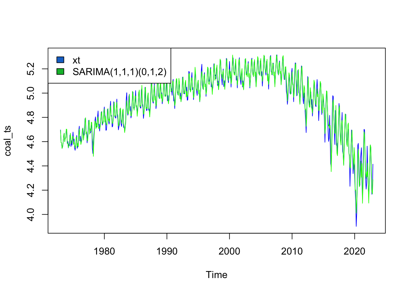
Series: coal_ts
ARIMA(1,1,1)(0,1,2)[12]

Coefficients:
         ar1      ma1     sma1     sma2
      0.7153  -0.9330  -0.7101  -0.0771
s.e.  0.0468   0.0262   0.0463   0.0433

sigma^2 = 0.001933:  log likelihood = 997.03
AIC=-1984.07   AICc=-1983.97   BIC=-1962.19

Training set error measures:
                      ME       RMSE        MAE         MPE      MAPE      MASE
Training set -0.00220553 0.04333907 0.02966952 -0.05188677 0.6181671 0.5017093
                    ACF1
Training set -0.02887885
Hydrocarbon
The SARIMA model that minimizes AIC and AICc is SARIMA(1,1,2)(0,1,1)
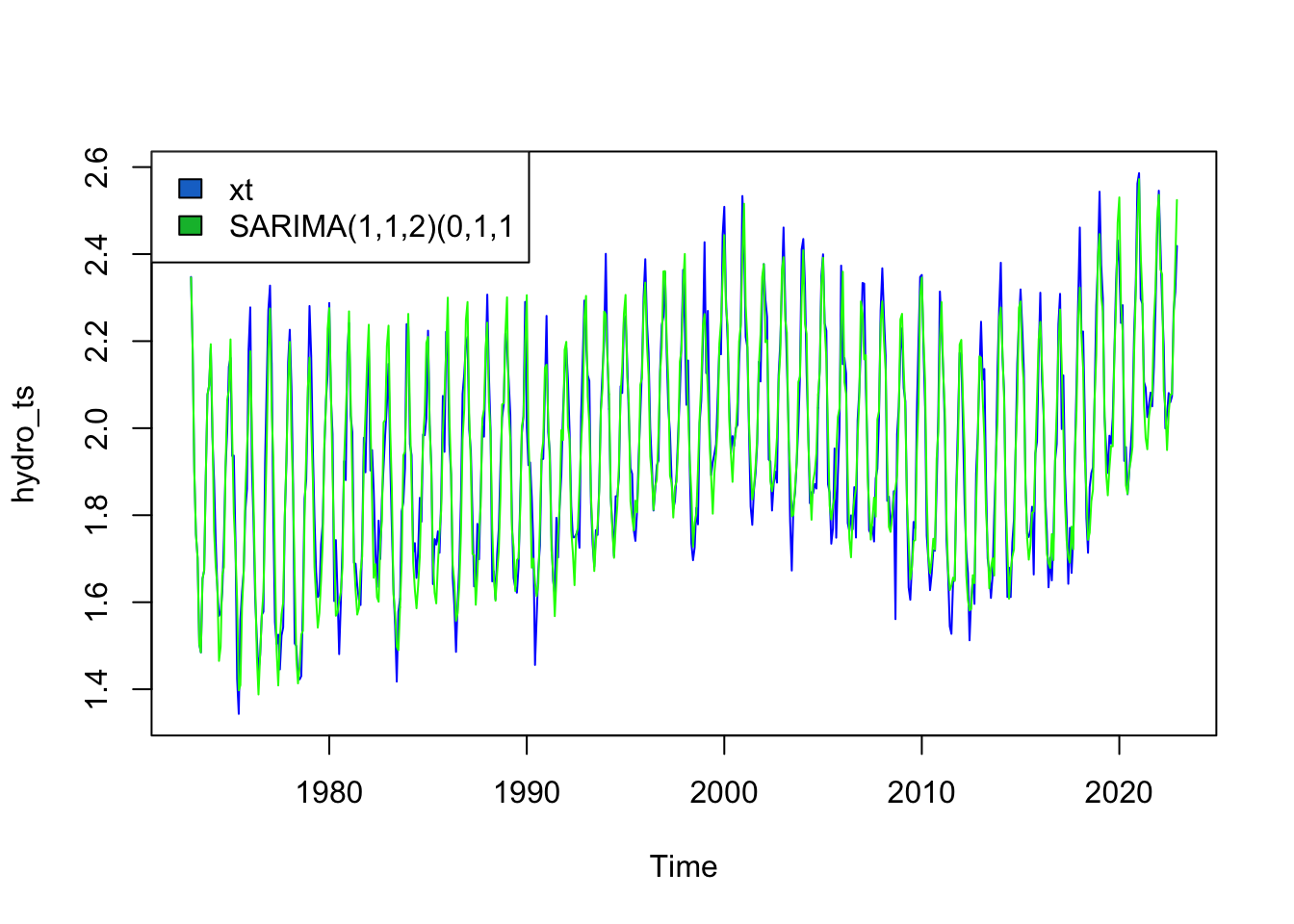
Series: hydro_ts
ARIMA(1,1,2)(0,1,1)[12]

Coefficients:
         ar1      ma1     ma2     sma1
      0.6838  -1.2657  0.3178  -0.8718
s.e.  0.1003   0.1177  0.0981   0.0302

sigma^2 = 0.005473:  log likelihood = 688.21
AIC=-1366.43   AICc=-1366.32   BIC=-1344.55

Training set error measures:
                      ME       RMSE        MAE        MPE     MAPE      MASE
Training set 0.003801311 0.07292737 0.05689759 0.09963854 2.964171 0.6705054
                    ACF1
Training set 0.002831291
Natural Gas
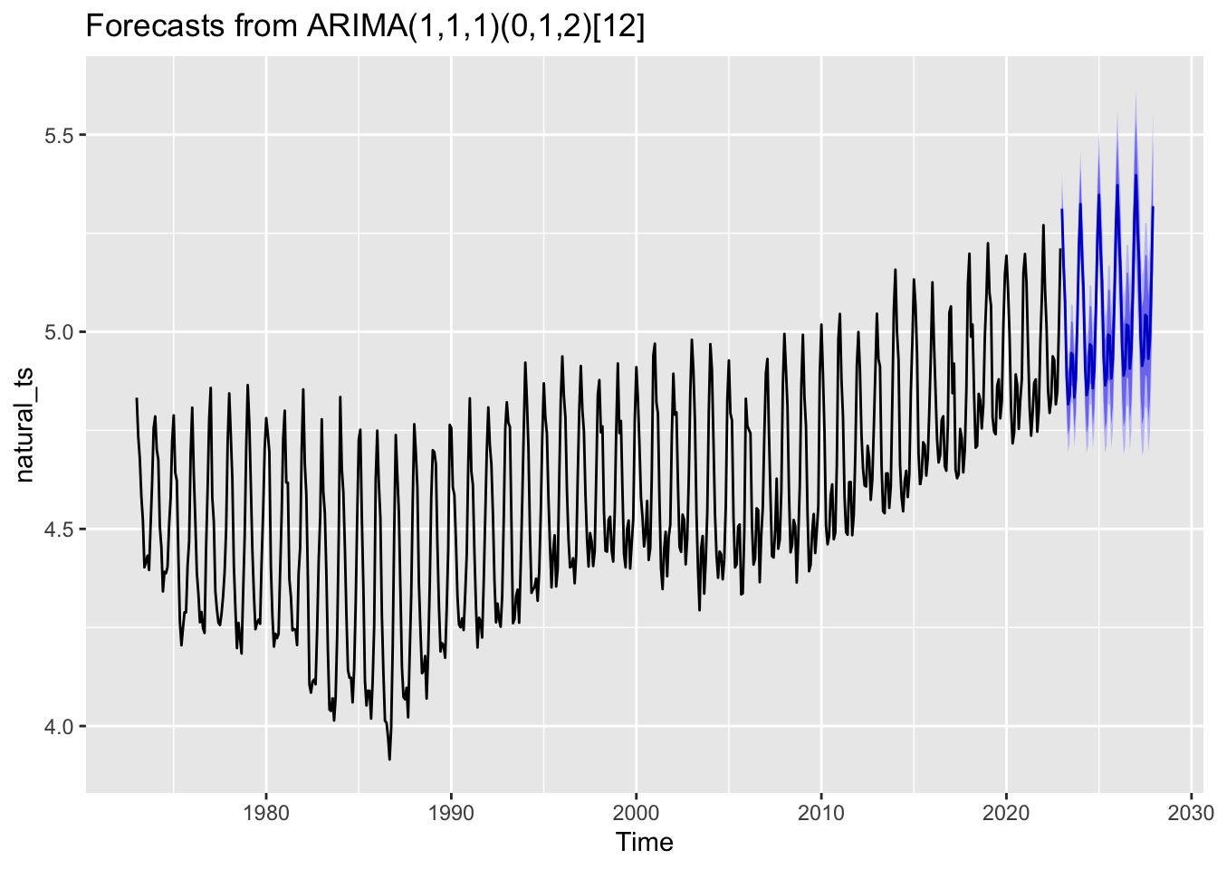
The SARIMA model that minimizes AIC and AICc is SARIMA(1,1,1)(0,1,2)
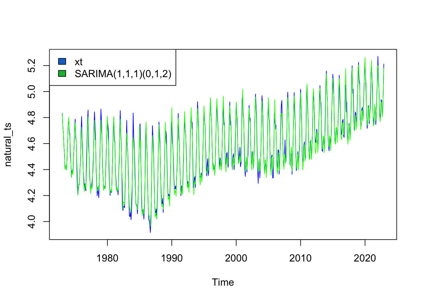
Series: natural_ts
ARIMA(1,1,1)(0,1,2)[12]

Coefficients:
         ar1      ma1     sma1     sma2
      0.5435  -0.9253  -0.6784  -0.0909
s.e.  0.0438   0.0183   0.0439   0.0449

sigma^2 = 0.002253:  log likelihood = 952.42
AIC=-1894.85   AICc=-1894.75   BIC=-1872.97

Training set error measures:
                      ME       RMSE        MAE        MPE      MAPE     MASE
Training set 0.002460763 0.04678813 0.03593403 0.04625378 0.7828864 0.655979
                    ACF1
Training set 0.004392229
Petroleum
The SARIMA model that minimizes AIC, BIC, and AICc is SARIMA(0,1,1)(1,1,1)
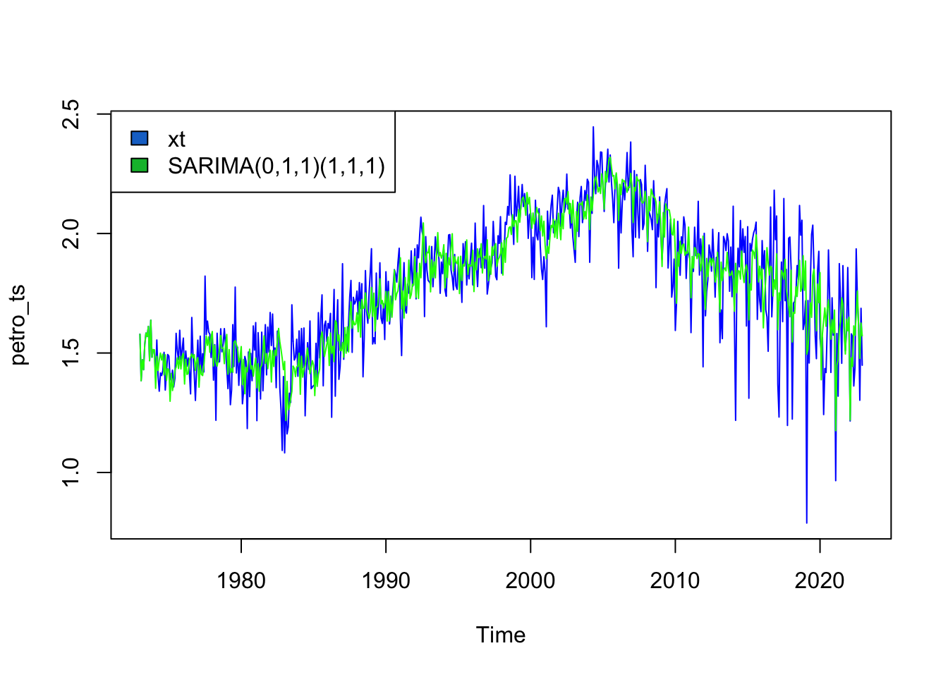
Series: petro_ts
ARIMA(0,1,1)(1,1,1)[12]

Coefficients:
          ma1     sar1     sma1
      -0.8639  -0.1659  -0.8360
s.e.   0.0226   0.0469   0.0289

sigma^2 = 0.02081:  log likelihood = 295.28
AIC=-582.57   AICc=-582.5   BIC=-565.07

Training set error measures:
                       ME     RMSE       MAE        MPE     MAPE      MASE
Training set -0.001821531 0.142328 0.1073413 -0.7744743 6.447119 0.6979237
                   ACF1
Training set 0.01685106
5) Fit a SARIMA(p,d,q)(P,D,Q) model using auto.arima()
Coal
Series: coal_ts
ARIMA(1,1,1)(0,1,2)[12]

Coefficients:
         ar1      ma1     sma1     sma2
      0.7153  -0.9330  -0.7101  -0.0771
s.e.  0.0468   0.0262   0.0463   0.0433

sigma^2 = 0.001933:  log likelihood = 997.03
AIC=-1984.07   AICc=-1983.97   BIC=-1962.19
The model chosen was ARIMA(1,1,1)(0,1,2) which is the same as I chose via manual fitting!
Hydrocarbon
Series: hydro_ts
ARIMA(2,0,1)(2,1,2)[12] with drift

Coefficients:
         ar1      ar2      ma1     sar1     sar2     sma1     sma2  drift
      1.2627  -0.2778  -0.8241  -0.4107  -0.1018  -0.4327  -0.3460  6e-04
s.e.  0.0810   0.0733   0.0587   0.2109   0.0598   0.2094   0.1941  5e-04

sigma^2 = 0.005468:  log likelihood = 693.26
AIC=-1368.51   AICc=-1368.2   BIC=-1329.12
The model chosen was ARIMA(2,0,1)(0,1,2) which is different from my chosen model of ARIMA(1,1,2)(0,1,1).
Natural Gas
Series: natural_ts
ARIMA(2,1,1)(1,1,1)[12]

Coefficients:
         ar1      ar2      ma1    sar1     sma1
      0.5500  -0.0177  -0.9225  0.1084  -0.7961
s.e.  0.0468   0.0442   0.0201  0.0573   0.0396

sigma^2 = 0.002258:  log likelihood = 952.25
AIC=-1892.51   AICc=-1892.36   BIC=-1866.26
The model chosen was ARIMA(2,1,1)(1,1,1) which was different from my chosen model of ARIMA(1,1,1)(0,1,2).
Petroleum
Series: petro_ts
ARIMA(0,1,1)(0,0,2)[12]

Coefficients:
          ma1    sma1    sma2
      -0.8842  0.0798  0.1886
s.e.   0.0214  0.0443  0.0378

sigma^2 = 0.0244:  log likelihood = 262.41
AIC=-516.83   AICc=-516.76   BIC=-499.24
The model chosen was ARIMA(0,1,1)(0,0,2) which was slightly different from my chosen model of ARIMA(0,1,1)(1,1,1). The seasonal effects were handled differently by auto.arima()
6) Forecast
Forecasting CO2 Emissions by source for the next 5 years
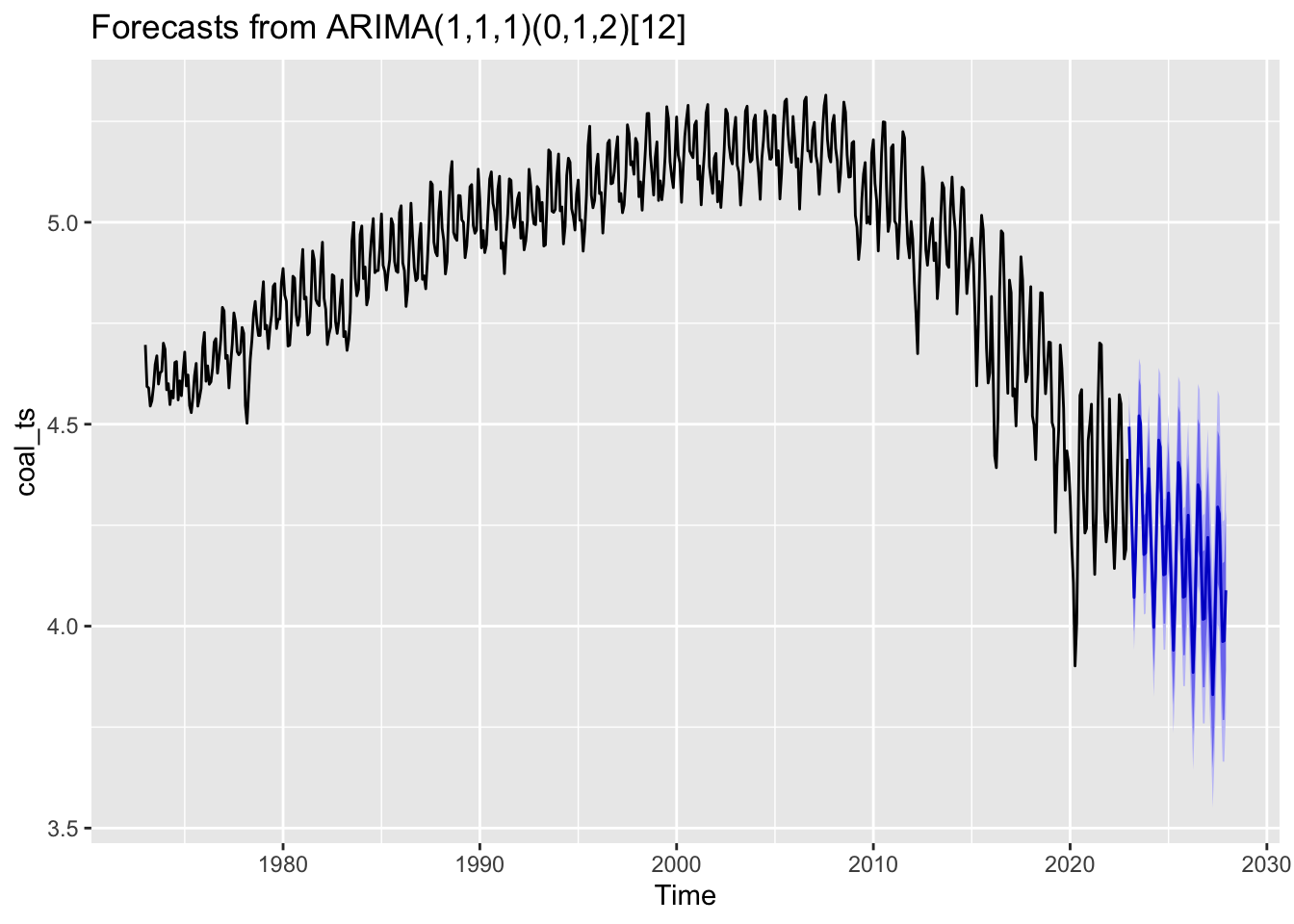
Coal
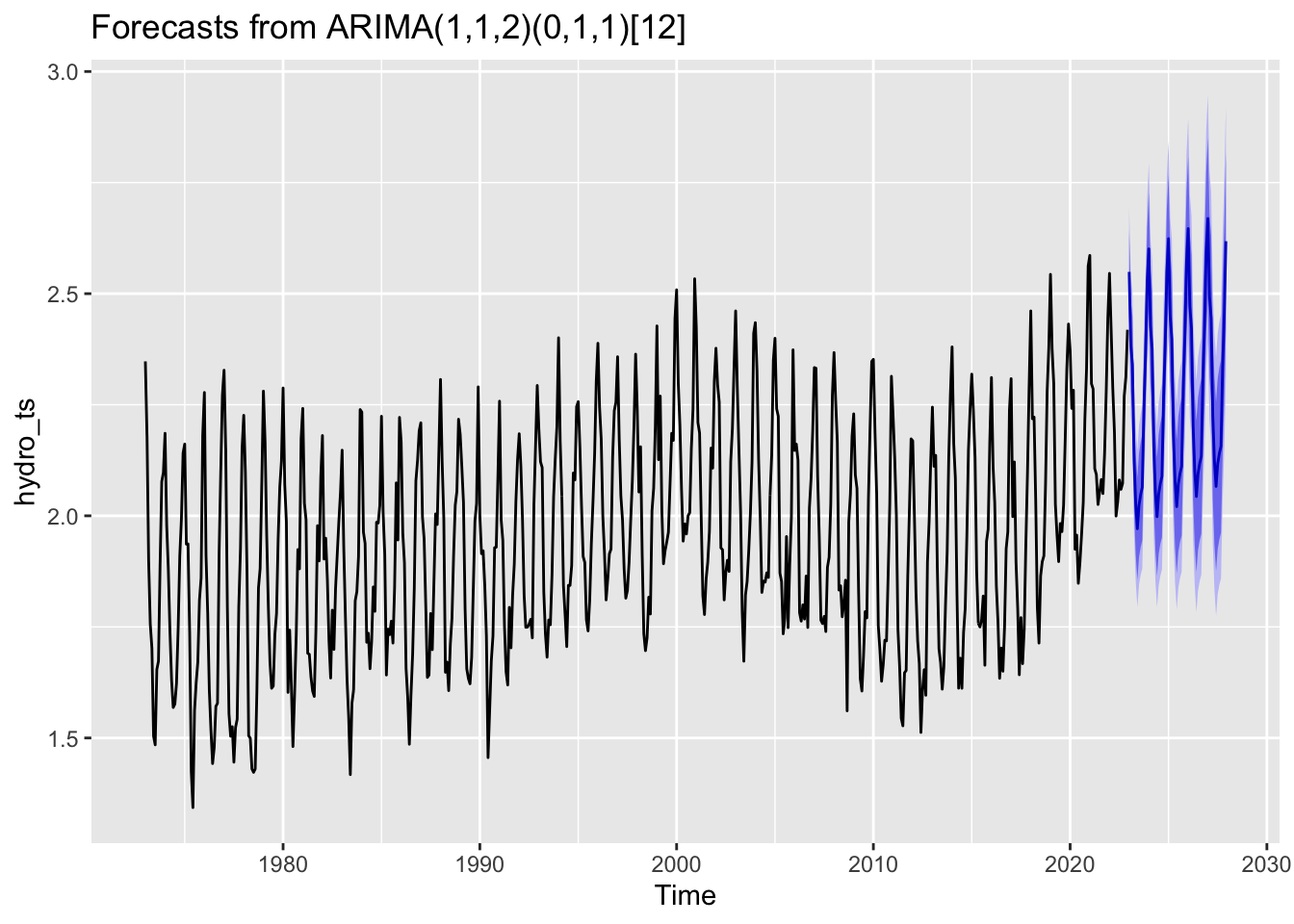
Hydrocarbon
Natural Gas
Petroleum
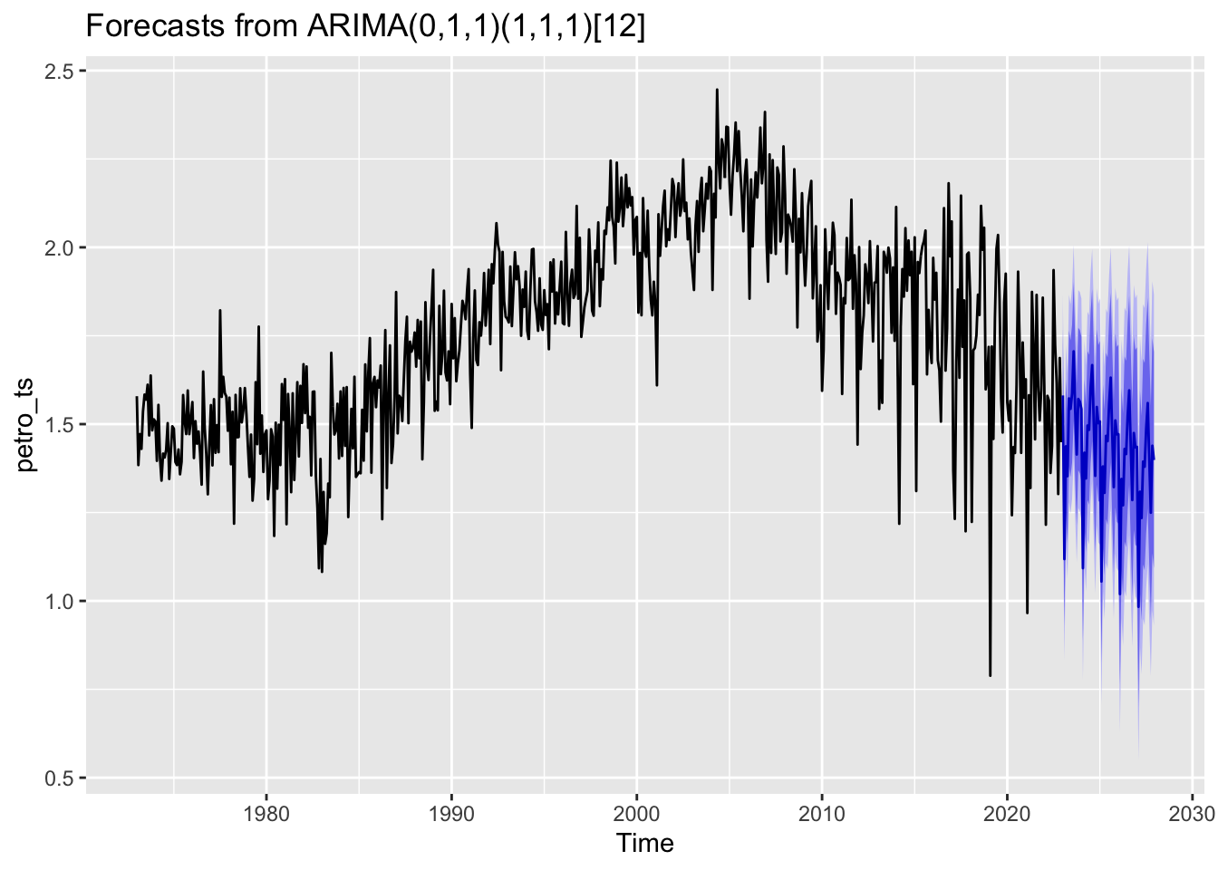
According to our models, coal emissions are expected to continue their steep downwards trend over the next 5 years, while CO2 Emissions from Petroleum are also expected to decrease over the next 5 years - albeit slightly less dramatically. CO2 emissions from both Hydrocarbon Gas and Natural Gas are forecasted to increase over the next 5 years.
7) Benchmark
Compare the models to baseline benchmark methods to ensure they’re performing above.
Coal
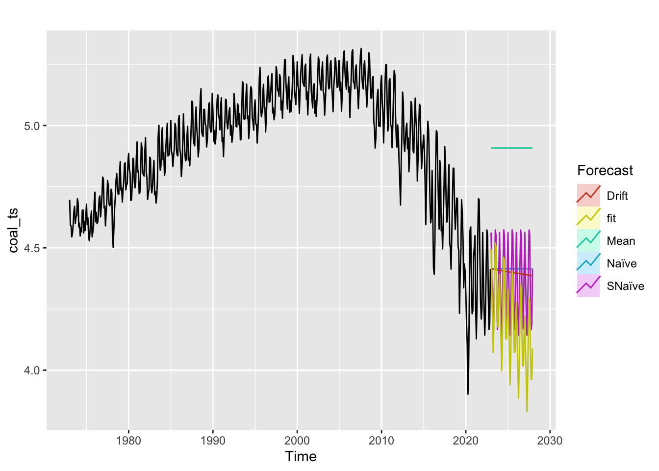
All benchmark methods predict CO2 emissions to stay steady or increase over the next 5 years. It looks like our model outperforms the benchmark methods.
Hydrocarbon
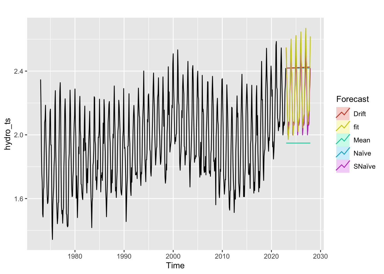
Both fit and seasonal naive methods predict an upward trend in CO2 emissions, with seasonal variation preserved. Drift, mean, and naive methods predict constant emissions and our model is far better.
Natural Gas
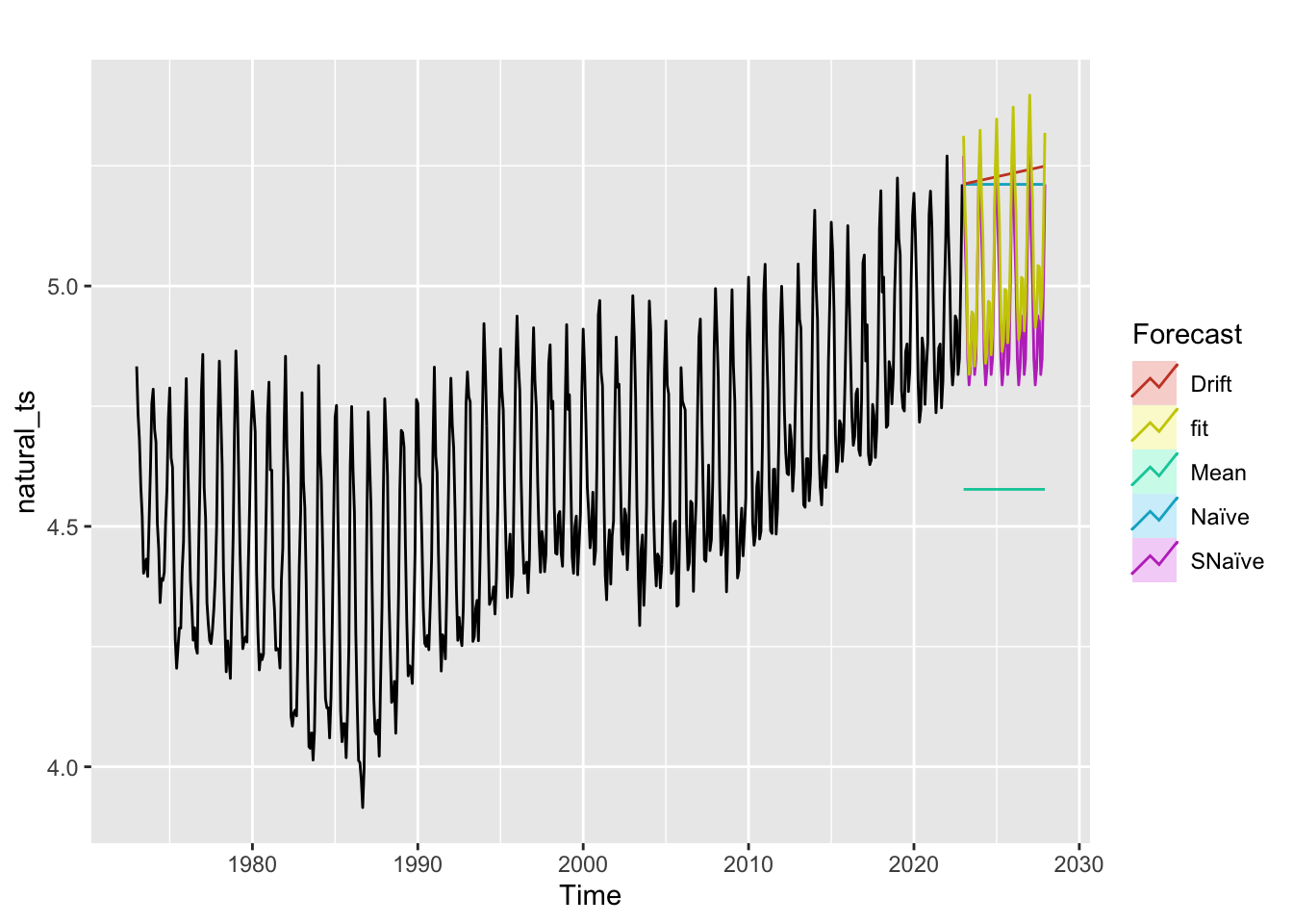
Drift, Mean and Naive methods predict constant emissions over the next 5 years. Seasonal naive predicts increasing CO2 emissions with seasonal variation, but the fit outperforms seasonal naive and it follows the trend slightly better.
Petroleum
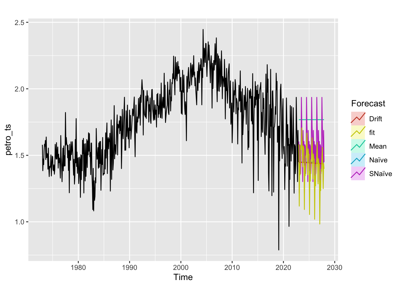
The fit and seasonal naive preserve the seasonal variation but the model fit forecasts decreasing CO2 emissions (following the trend) and seasonal naive predicts increasing seasonal variation. Drift, mean, and naive benchmark methods again severely underperform.
8) Seasonal Cross Validation
1 Step Ahead
Coal ARIMA(1,1,1)(0,1,2) for both auto.arima() and manual fitting.
 [1] 0.04619373 0.04570981 0.04725047 0.04745566 0.04854170 0.04904679
 [7] 0.04993501 0.05057058 0.05137274 0.05206507 0.05282980 0.05354680
[13] 0.05429527 0.05502300 0.05576439 0.05649678 0.05723510 0.05796952
[19] 0.05870651 0.05944180 0.06017821 0.06091388 0.06165004 0.06238588
[25] 0.06312193 0.06430790 0.06632118 0.06833454 0.07034785 0.07236119
[31] 0.07437451 0.07638784 0.07840117 0.08041450 0.08242783 0.08444115
[37] 0.08645448 0.08846781 0.09048114 0.09249447 0.09450779 0.09652112
[43] 0.09853445 0.10054778 0.10256111 0.10457443 0.10658776 0.10860109
[49] 0.11061442 0.11262775 0.11464107 0.11665440 0.11866773 0.12068106
[55] 0.12269439 0.12470771 0.12672104 0.12873437 0.13074770 0.13276103
Hydrocarbon ARIMA(2,0,1)(0,1,2) for auto.arima() and ARIMA(1,1,2)(0,1,1) from manual fitting.
 [1] 0.07974090 0.21231107 0.34844198 0.43904916 0.46729056 0.43355642
 [7] 0.35332484 0.25158786 0.15561699 0.08803235 0.06183177 0.07836086
[13] 0.12837006 0.19553350 0.26127758 0.30958432 0.33059942 0.32230591
[19] 0.29008470 0.24452063 0.19819837 0.16239099 0.14446263 0.14653472
[25] 0.16559137 0.19482700 0.22575927 0.25050036 0.26361288 0.26314655
[31] 0.25069987 0.23060751 0.20855614 0.19003452 0.17901631 0.17716960
[37] 0.18372372 0.19594748 0.21004964 0.22223107 0.22961376 0.23083438
[43] 0.22619708 0.21740091 0.20695879 0.19748680 0.19105279 0.18873644
[49] 0.19048299 0.19525160 0.20138694 0.20709667 0.21090569 0.21197878
[55] 0.21024853 0.20634046 0.20133780 0.19646233 0.19275939 0.19086346
[1] 0.08971719 0.09637873 0.09879890 0.09967010 0.09997514 0.10007317
[7] 0.10009549 0.10009014 0.10007468 0.10005553 0.10003503 0.10001403
[13] 0.09999286 0.09997162 0.09995036 0.09992909 0.09990782 0.09988655
[19] 0.09986527 0.09984400 0.09982272 0.09980145 0.09978017 0.09975890
[25] 0.09973762 0.09971635 0.09969508 0.09967380 0.09965253 0.09963125
[31] 0.09960998 0.09958870 0.09956743 0.09954615 0.09952488 0.09950361
[37] 0.09948233 0.09946106 0.09943978 0.09941851 0.09939723 0.09937596
[43] 0.09935468 0.09933341 0.09931213 0.09929086 0.09926959 0.09924831
[49] 0.09922704 0.09920576 0.09918449 0.09916321 0.09914194 0.09912066
[55] 0.09909939 0.09907812 0.09905684 0.09903557 0.09901429 0.09899302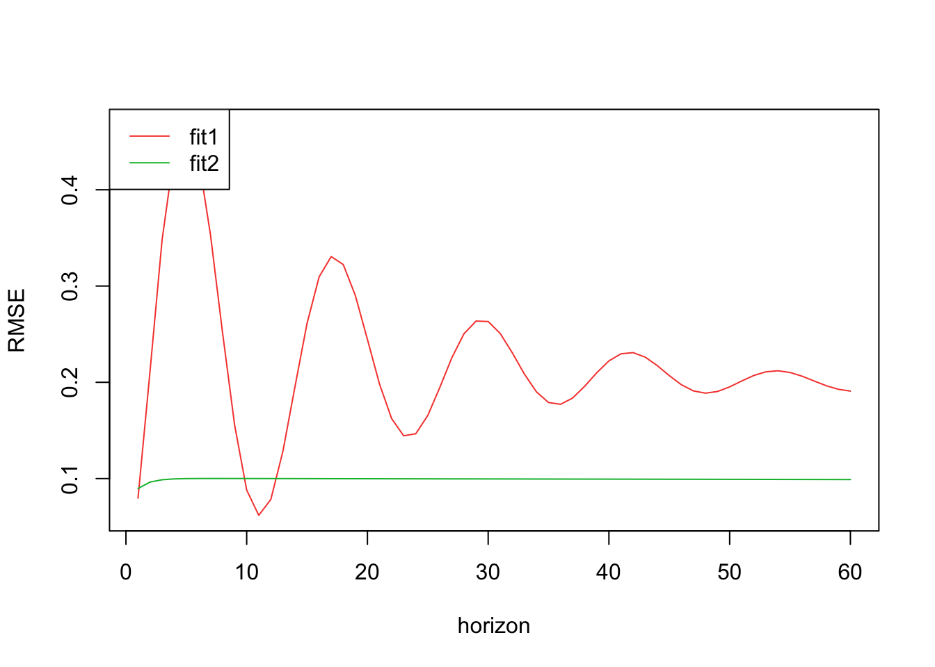
From this, it appears that ARIMA(2,0,1)(0,1,2) has much more variable RMSE, but overall is a better fit model
Natural gas ARIMA(2,1,1)(1,1,1) for auto.arima() and ARIMA(1,1,1)(0,1,2) from manual fitting.
 [1] 0.05279172 0.17922373 0.31912281 0.42672446 0.48067602 0.48246156
 [7] 0.44856163 0.40070412 0.35771745 0.33088375 0.32303682 0.33045894
[13] 0.34610679 0.36277882 0.37530316 0.38141445 0.38148409 0.37755569
[19] 0.37219683 0.36756755 0.36491146 0.36448378 0.36579586 0.36800119
[25] 0.37026257 0.37199741 0.37296817 0.37324094 0.37306752 0.37275048
[31] 0.37253697 0.37256333 0.37285056 0.37333544 0.37391662 0.37449699
[37] 0.37501116 0.37543457 0.37577755 0.37607094 0.37635031 0.37664385
[43] 0.37696642 0.37731945 0.37769487 0.37808058 0.37846534 0.37884186
[49] 0.37920762 0.37956414 0.37991518 0.38026490 0.38061650 0.38097161
[55] 0.38133027 0.38169145 0.38205372 0.38241579 0.38277683 0.38313660
[1] 0.05169864 0.08091653 0.09517965 0.10221910 0.10576896 0.10763298
[7] 0.10868248 0.10933841 0.10980416 0.11017801 0.11050744 0.11081540
[13] 0.11111299 0.11140556 0.11169571 0.11198468 0.11227308 0.11256121
[19] 0.11284921 0.11313715 0.11342505 0.11371294 0.11400082 0.11428870
[25] 0.11457658 0.11486445 0.11515233 0.11544020 0.11572808 0.11601595
[31] 0.11630383 0.11659170 0.11687958 0.11716745 0.11745533 0.11774320
[37] 0.11803108 0.11831895 0.11860683 0.11889470 0.11918258 0.11947045
[43] 0.11975833 0.12004620 0.12033408 0.12062195 0.12090983 0.12119770
[49] 0.12148558 0.12177345 0.12206133 0.12234920 0.12263708 0.12292495
[55] 0.12321283 0.12350070 0.12378858 0.12407645 0.12436433 0.12465220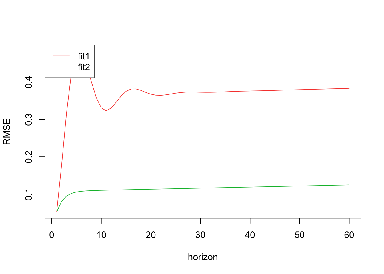
From this analysis, it looks like ARIMA(2,1,1)(1,1,1) is a better fit model.
Petroleum ARIMA(0,1,1)(0,0,2) for auto.arima() and ARIMA(0,1,1)(1,1,1) from manual fitting.
 [1] 0.08598773 0.08658462 0.08718152 0.08777841 0.08837531 0.08897220
 [7] 0.08956909 0.09016599 0.09076288 0.09135978 0.09195667 0.09255356
[13] 0.09315046 0.09374735 0.09434425 0.09494114 0.09553803 0.09613493
[19] 0.09673182 0.09732872 0.09792561 0.09852250 0.09911940 0.09971629
[25] 0.10031319 0.10091008 0.10150697 0.10210387 0.10270076 0.10329766
[31] 0.10389455 0.10449144 0.10508834 0.10568523 0.10628213 0.10687902
[37] 0.10747591 0.10807281 0.10866970 0.10926660 0.10986349 0.11046038
[43] 0.11105728 0.11165417 0.11225107 0.11284796 0.11344485 0.11404175
[49] 0.11463864 0.11523554 0.11583243 0.11642932 0.11702622 0.11762311
[55] 0.11822001 0.11881690 0.12041907 0.12202312 0.12362717 0.12523122
[1] 0.08598773 0.08658462 0.08718152 0.08777841 0.08837531 0.08897220
[7] 0.08956909 0.09016599 0.09076288 0.09135978 0.09195667 0.09255356
[13] 0.09315046 0.09374735 0.09434425 0.09494114 0.09553803 0.09613493
[19] 0.09673182 0.09732872 0.09792561 0.09852250 0.09911940 0.09971629
[25] 0.10031319 0.10091008 0.10150697 0.10210387 0.10270076 0.10329766
[31] 0.10389455 0.10449144 0.10508834 0.10568523 0.10628213 0.10687902
[37] 0.10747591 0.10807281 0.10866970 0.10926660 0.10986349 0.11046038
[43] 0.11105728 0.11165417 0.11225107 0.11284796 0.11344485 0.11404175
[49] 0.11463864 0.11523554 0.11583243 0.11642932 0.11702622 0.11762311
[55] 0.11822001 0.11881690 0.12041907 0.12202312 0.12362717 0.12523122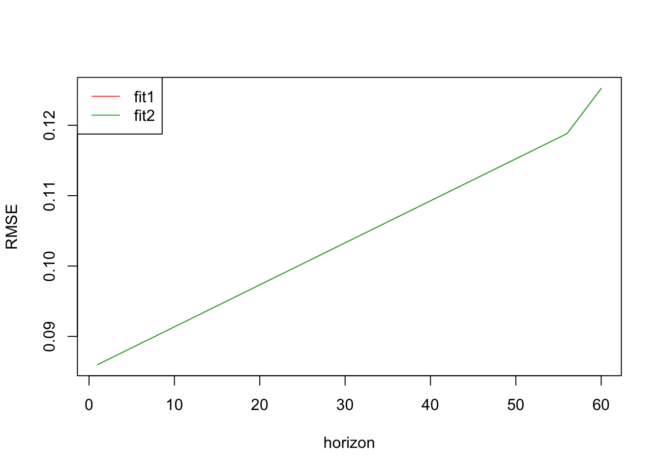
From this analysis, it looks like both models perform similarly and have the same RMSE.
12 steps ahead forecast
Coal ARIMA(1,1,1)(0,1,2) for both auto.arima() and manual fitting.
[1] 525[1] 0.3327111Hydrocarbon ARIMA(2,0,1)(0,1,2) for auto.arima() and ARIMA(1,1,2)(0,1,1) from manual fitting.
[1] 525[1] 0.4455012[1] 0.4738333From this analysis, ARIMA(2,0,1)(0,1,2) from auto.arima() has a much lower RMSE.
Natural gas ARIMA(2,1,1)(1,1,1) for auto.arima() and ARIMA(1,1,1)(0,1,2) from manual fitting.
[1] 525[1] 0.4328701[1] 0.4238351From this analysis, ARIMA(1,1,1)(0,1,2) from manual fitting has a much lower RMSE and is a better fit model for this data.
Petroleum ARIMA(0,1,1)(0,0,2) for auto.arima() and ARIMA(0,1,1)(1,1,1) from manual fitting.
[1] 525[1] 0.367206[1] 0.367206From this analysis, it appears that both models perform the same and have the same RMSE. Either is a valid model to work with.
Source code for the above analysis: Github