Coal observations:  (649, 1)
Hydro observations:  (649, 1)
Natural Gas observations:  (649, 1)
Petroleum observations: (649, 1)Deep Learning for Time Series

Using univariate time series, I here use deep learning to extract insights about energy in the United States. I use a Recurrent Neural Network (RNN), a Gated Recurrent Unit (GRU) network, and a Long-Short Term Memory Network (LSTM) to make future predictions related to CO2 Emissions. This analysis is in Python.
NOTE: NN analysis on CO2 emissions data only due to sample size limitations. Because all the other datasets are on a yearly frequency we have a maximum of 50 datapoints per energy source - not enough to build a model with.
Packages used: pandas, numpy, plotly, matplotlib, tensorflow, keras, sklearn
CO2 Emissions
Broken down by emissions by Coal, Hydro, Natural Gas, Petroleum, and Total source.
Coal
Split data into training and testing data
And visualize split!
Training data size:  (519,)
Test data size:  (130,)
Reformat data into required shape
Required shape = (samples, time, features)
Model 1 = RNN
Model architecture
Model: "sequential"
_________________________________________________________________
 Layer (type)                Output Shape              Param #
=================================================================
 simple_rnn (SimpleRNN)      (None, 3)                 15

 dense (Dense)               (None, 1)                 4

=================================================================
Total params: 19
Trainable params: 19
Non-trainable params: 0
_________________________________________________________________
2023-04-30 23:41:10.947038: I tensorflow/core/platform/cpu_feature_guard.cc:193] This TensorFlow binary is optimized with oneAPI Deep Neural Network Library (oneDNN) to use the following CPU instructions in performance-critical operations: SSE4.1 SSE4.2 AVX AVX2 FMA
To enable them in other operations, rebuild TensorFlow with the appropriate compiler flags.Plot training and validation loss (MSE)
1/2 [==============>...............] - ETA: 0s2/2 [==============================] - 0s 2ms/step
1/1 [==============================] - ETA: 0s1/1 [==============================] - 0s 17ms/step
(51, 9, 1) (51,) (51,) (12, 9, 1) (12,) (12,)
(51,) (51,)
0.035081297
0.02046974
Train MSE = 0.03508 RMSE = 0.18730
Test MSE = 0.02047 RMSE = 0.14307
Forecasting - next 5 years (60 months)
1/1 [==============================] - ETA: 0s1/1 [==============================] - 0s 18ms/step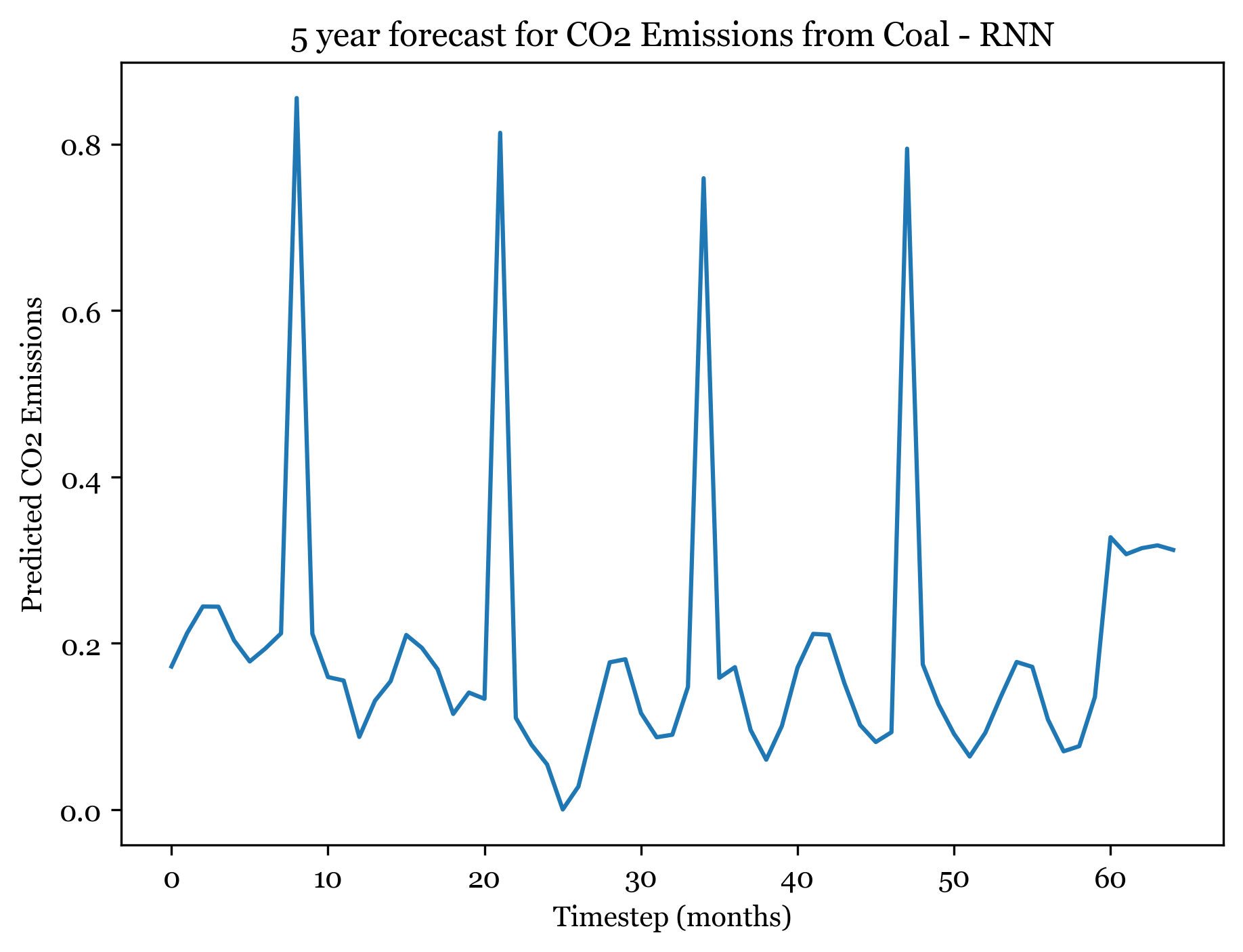
Model 2 - GRU
Model Architecture
Model: "sequential_1"
_________________________________________________________________
 Layer (type)                Output Shape              Param #
=================================================================
 gru (GRU)                   (None, 3)                 54

 dense_1 (Dense)             (None, 1)                 4

=================================================================
Total params: 58
Trainable params: 58
Non-trainable params: 0
_________________________________________________________________
Plot training and validation loss
1/2 [==============>...............] - ETA: 0s2/2 [==============================] - 0s 2ms/step
1/1 [==============================] - ETA: 0s1/1 [==============================] - 0s 16ms/step
(51, 9, 1) (51,) (51,) (5, 9, 1) (5,) (5,)
(51,) (51,)
0.03370281
0.034062225
Train MSE = 0.03370 RMSE = 0.18358
Test MSE = 0.03406 RMSE = 0.18456
Forecasting - next 5 years (60 months)
1/1 [==============================] - ETA: 0s1/1 [==============================] - 0s 18ms/step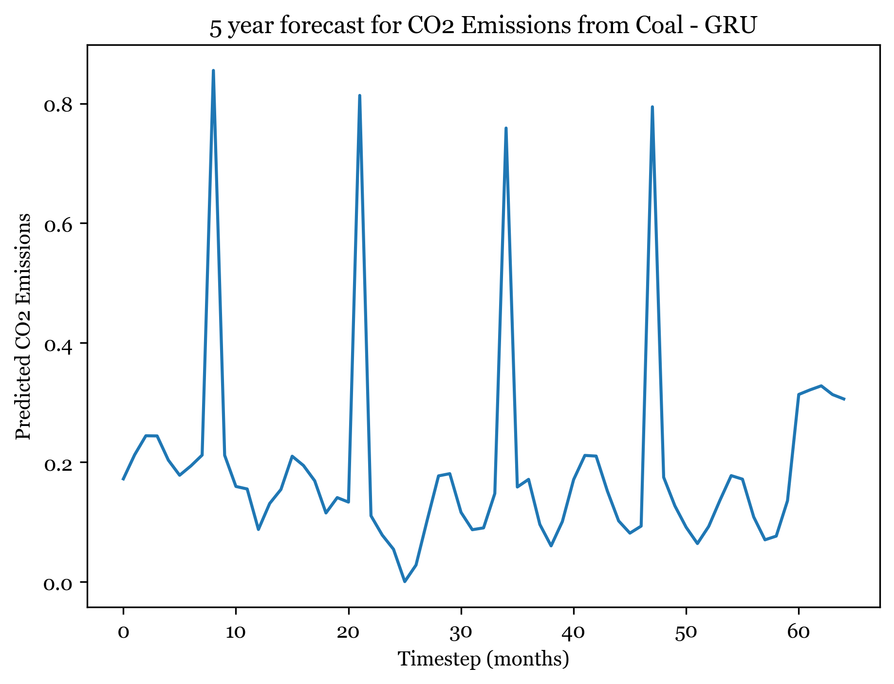
Model 3 - LSTM
Model Architecture
Model: "sequential_2"
_________________________________________________________________
 Layer (type)                Output Shape              Param #
=================================================================
 lstm (LSTM)                 (None, 3)                 60

 dense_2 (Dense)             (None, 1)                 4

=================================================================
Total params: 64
Trainable params: 64
Non-trainable params: 0
_________________________________________________________________
Plot training and validation loss
1/2 [==============>...............] - ETA: 0s2/2 [==============================] - 0s 3ms/step
1/1 [==============================] - ETA: 0s1/1 [==============================] - 0s 18ms/step
(51, 9, 1) (51,) (51,) (5, 9, 1) (5,) (5,)
(51,) (51,)
0.034197398
0.019271672
Train MSE = 0.03420 RMSE = 0.18493
Test MSE = 0.01927 RMSE = 0.13882
Forecasting - next 5 years (60 months)
1/1 [==============================] - ETA: 0s1/1 [==============================] - 0s 23ms/step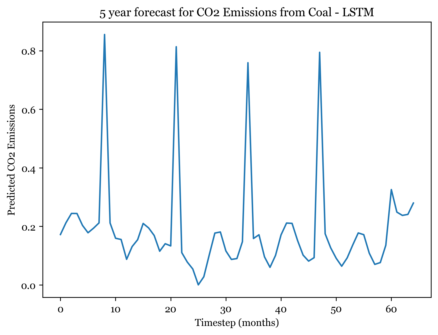
Discussion
For predicting CO2 emissions from coal, the training RMSE are:
1) RNN - 0.18039
2) GRU - 0.18312
3) LSTM - 0.18691
And the test RMSE are:
1) RNN - 0.12964
2) GRU - 0.19448
3) LSTM - 0.14685
Thus, the RNN minimized RMSE for both training and validation predictions, while the GRU model overfit the data. Regularization is a technique used in ANNs to prevent overfitting and improve generalization performance. L2 regularization was used here, which adds a penalty term to the loss function that is proportional to the sum of the squares of the weights in the network. It was decently important here - without L2 regularization the test RMSE for RNN, GRU, and LSTM models were all over 0.2 which is much higher than their regularized RMSE above.
Forecasting here worked better than expected. For all three models I forecasted the next 5 years (60) months, and the forecasted plots appear to mimic the seasonality and spikes of the previous 30 years. Across all three models, the first 3-4 years are well forecasted and display the expected spikes in emissions during the summer. However, by year 5 forecast weakens and the nuance and variation in the trend is smaller.
The ARIMA(1,1,1)(0,1,2) forecast shared the same seasonality, but exhibited a downwards trend. The ANN models also exhibit a slight downward trend, but are far more consistent over time. The RNSE from the ARIMA model was 0.0433, significantly smaller than the ANN RMSE. With more model tuning the ANN could likely outperform the ARIMA model.
Hydro
Split data into training and testing data
And visualize split!
Training data size:  (519,)
Test data size:  (130,)
Reformat data into required shape
Required shape = (samples, time, features)
Model 1 = RNN
Model architecture
Model: "sequential_3"
_________________________________________________________________
 Layer (type)                Output Shape              Param #
=================================================================
 simple_rnn_1 (SimpleRNN)    (None, 3)                 15

 dense_3 (Dense)             (None, 1)                 4

=================================================================
Total params: 19
Trainable params: 19
Non-trainable params: 0
_________________________________________________________________
Plot training and validation loss (MSE)
1/2 [==============>...............] - ETA: 0s2/2 [==============================] - 0s 2ms/step
1/1 [==============================] - ETA: 0s1/1 [==============================] - 0s 15ms/step
(51, 9, 1) (51,) (51,) (12, 9, 1) (12,) (12,)
(51,) (51,)
0.04613612
0.00695966
Train MSE = 0.04614 RMSE = 0.21479
Test MSE = 0.00696 RMSE = 0.08342
Forecasting - next 5 years (60 months)
1/1 [==============================] - ETA: 0s1/1 [==============================] - 0s 16ms/step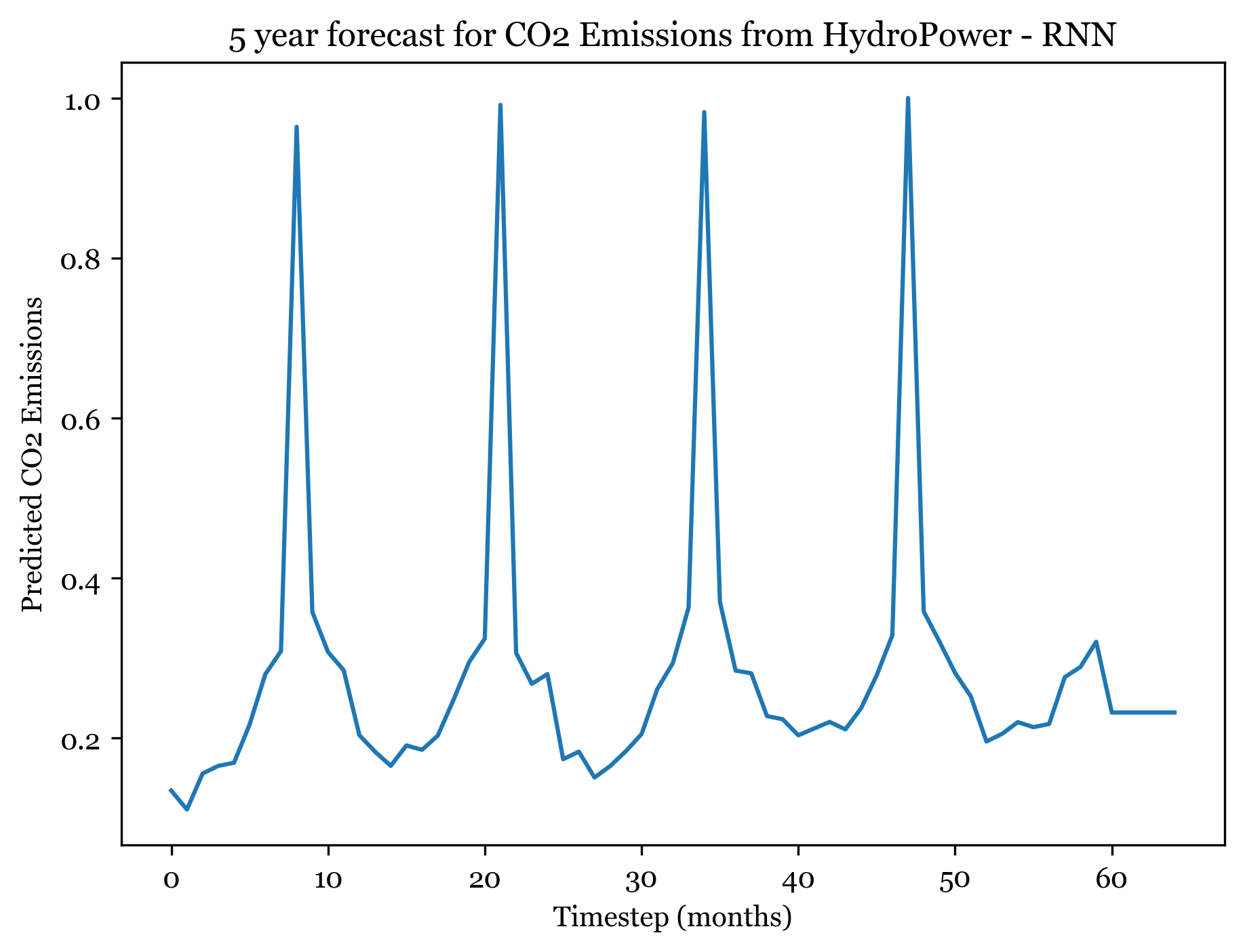
Model 2 - GRU
Model Architecture
Model: "sequential_4"
_________________________________________________________________
 Layer (type)                Output Shape              Param #
=================================================================
 gru_1 (GRU)                 (None, 3)                 54

 dense_4 (Dense)             (None, 1)                 4

=================================================================
Total params: 58
Trainable params: 58
Non-trainable params: 0
_________________________________________________________________
Plot training and validation loss
1/2 [==============>...............] - ETA: 0s2/2 [==============================] - 0s 3ms/step
1/1 [==============================] - ETA: 0s1/1 [==============================] - 0s 22ms/step
(51, 9, 1) (51,) (51,) (5, 9, 1) (5,) (5,)
(51,) (51,)
0.040841345
0.0011350267
Train MSE = 0.04084 RMSE = 0.20209
Test MSE = 0.00114 RMSE = 0.03369
Forecasting - next 5 years (60 months)
1/1 [==============================] - ETA: 0s1/1 [==============================] - 0s 18ms/step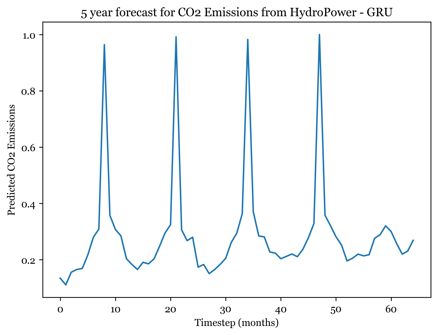
Model 3 - LSTM
Model Architecture
Model: "sequential_5"
_________________________________________________________________
 Layer (type)                Output Shape              Param #
=================================================================
 lstm_1 (LSTM)               (None, 3)                 60

 dense_5 (Dense)             (None, 1)                 4

=================================================================
Total params: 64
Trainable params: 64
Non-trainable params: 0
_________________________________________________________________
Plot training and validation loss
1/2 [==============>...............] - ETA: 0s2/2 [==============================] - 0s 3ms/step
1/1 [==============================] - ETA: 0s1/1 [==============================] - 0s 16ms/step
(51, 9, 1) (51,) (51,) (5, 9, 1) (5,) (5,)
(51,) (51,)
0.044831607
0.0038871728
Train MSE = 0.04483 RMSE = 0.21173
Test MSE = 0.00389 RMSE = 0.06235
Forecasting - next 5 years (60 months)
1/1 [==============================] - ETA: 0s1/1 [==============================] - 0s 17ms/step
Discussion
For predicting CO2 emissions from Hydro Power, the training RMSE are:
1) RNN - 0.17576
2) GRU - 0.19256
3) LSTM - 0.18912
And the test RMSE are:
1) RNN - 0.07061
2) GRU - 0.02567
3) LSTM - 0.07663
Thus, the RNN minimized RMSE for training predictions, but the GRU ANN produced the lowest test RMSE of the group. Test RMSE is significantly lower than training RMSE, so further analysis could investigate possible data leakage. Regularization again improved the model performance, by 0.04 points in the RMSE.
Forecasting here worked better than expected. For all three models I forecasted the next 5 years (60) months, and the forecasted plots appear to mimic the seasonality and spikes of the previous 30 years. Across all three models, the first 4 years are well forecasted and display the expected spikes in emissions during the summer. However, by year 5 forecast weakens and the nuance and variation in the trend is smaller.
The ARIMA(1,1,2)(0,1,1) forecast shared the same seasonality, but exhibited an upwards trend across all 5 years. The ANN models exhibit no trend (only seasonality). The RNSE from the ARIMA model was 0.07292737, significantly smaller than the ANN RMSE. With more model tuning the ANN could likely outperform the ARIMA model.
Natural Gas
Split data into training and testing data
And visualize split!
Training data size:  (519,)
Test data size:  (130,)
Reformat data into required shape
Required shape = (samples, time, features)
Model 1 = RNN
Model architecture
Model: "sequential_6"
_________________________________________________________________
 Layer (type)                Output Shape              Param #
=================================================================
 simple_rnn_2 (SimpleRNN)    (None, 3)                 15

 dense_6 (Dense)             (None, 1)                 4

=================================================================
Total params: 19
Trainable params: 19
Non-trainable params: 0
_________________________________________________________________
Plot training and validation loss (MSE)
1/2 [==============>...............] - ETA: 0s2/2 [==============================] - 0s 2ms/step
1/1 [==============================] - ETA: 0s1/1 [==============================] - 0s 19ms/step
(51, 9, 1) (51,) (51,) (12, 9, 1) (12,) (12,)
(51,) (51,)
0.03890586
0.0030931986
Train MSE = 0.03891 RMSE = 0.19725
Test MSE = 0.00309 RMSE = 0.05562
Forecasting - next 5 years (60 months)
1/1 [==============================] - ETA: 0s1/1 [==============================] - 0s 18ms/step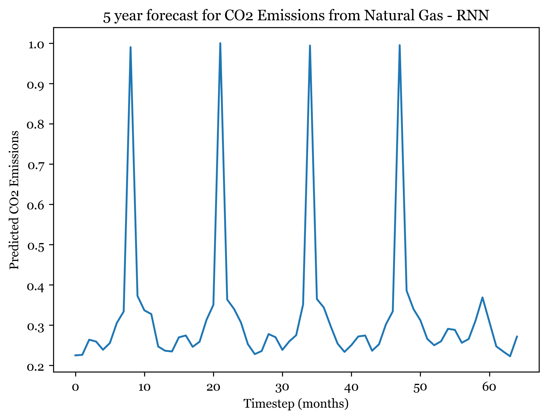
Model 2 - GRU
Model Architecture
Model: "sequential_7"
_________________________________________________________________
 Layer (type)                Output Shape              Param #
=================================================================
 gru_2 (GRU)                 (None, 3)                 54

 dense_7 (Dense)             (None, 1)                 4

=================================================================
Total params: 58
Trainable params: 58
Non-trainable params: 0
_________________________________________________________________
Plot training and validation loss
1/2 [==============>...............] - ETA: 0s2/2 [==============================] - 0s 3ms/step
1/1 [==============================] - ETA: 0s1/1 [==============================] - 0s 21ms/step
(51, 9, 1) (51,) (51,) (5, 9, 1) (5,) (5,)
(51,) (51,)
0.037088636
0.0038574208
Train MSE = 0.03709 RMSE = 0.19258
Test MSE = 0.00386 RMSE = 0.06211
Forecasting - next 5 years (60 months)
1/1 [==============================] - ETA: 0s1/1 [==============================] - 0s 22ms/step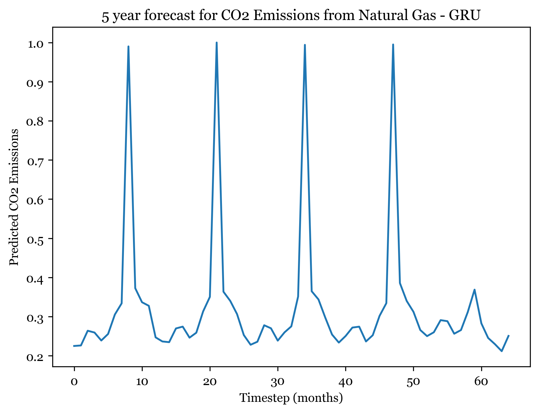
Model 3 - LSTM
Model Architecture
Model: "sequential_8"
_________________________________________________________________
 Layer (type)                Output Shape              Param #
=================================================================
 lstm_2 (LSTM)               (None, 3)                 60

 dense_8 (Dense)             (None, 1)                 4

=================================================================
Total params: 64
Trainable params: 64
Non-trainable params: 0
_________________________________________________________________
Plot training and validation loss
1/2 [==============>...............] - ETA: 0s2/2 [==============================] - 0s 3ms/step
1/1 [==============================] - ETA: 0s1/1 [==============================] - 0s 19ms/step
(51, 9, 1) (51,) (51,) (5, 9, 1) (5,) (5,)
(51,) (51,)
0.038007062
0.01997656
Train MSE = 0.03801 RMSE = 0.19495
Test MSE = 0.01998 RMSE = 0.14134
Forecasting - next 5 years (60 months)
1/1 [==============================] - ETA: 0s1/1 [==============================] - 0s 23ms/step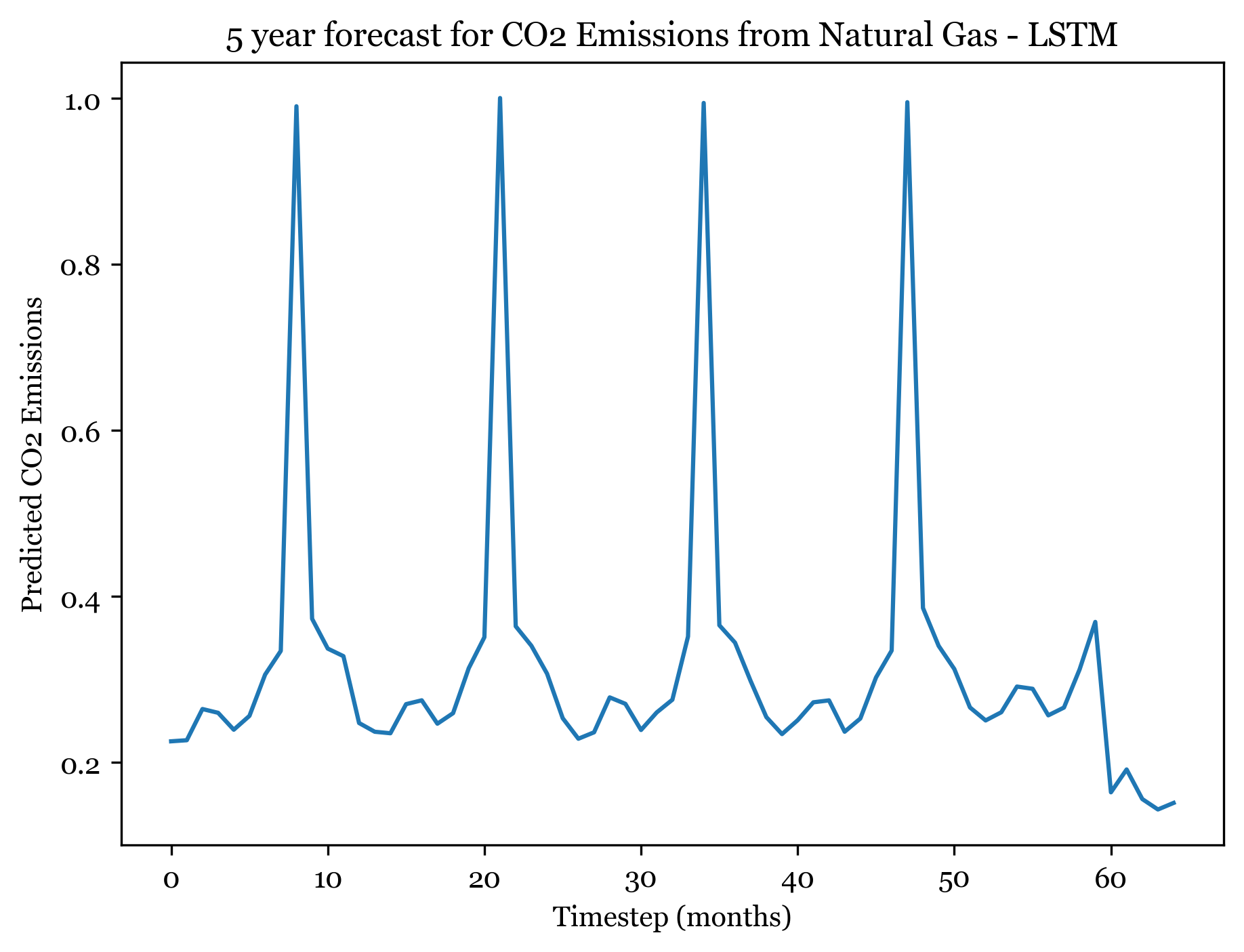
Discussion
For predicting CO2 emissions from Natural Gas, the training RMSE are:
1) RNN - 0.19666
2) GRU - 0.19114
3) LSTM - 0.18312
And the test RMSE are:
1) RNN - 0.05314
2) GRU - 0.07994
3) LSTM - 0.21063
Thus, the GRU model minimized RMSE for training predictions, while the RNN minimized RMSE for test predictions. Similarly to Hydro modeling, there is a pretty big difference between train and test RMSE for RNN and GRU models here. This could indicate data leakage and should be investigated via further analysis. The LSTM, on the other hand, appears to be overfitted as the test RMSE is higher than the train RMSE. Regularization again improved the model performance slightly, by 0.02 points in the RMSE.
Forecasting here worked better than expected. For all three models I forecasted the next 5 years (60) months, and the forecasted plots appear to mimic the seasonality and spikes of the previous 30 years. Across all three models, the first 4 years are well forecasted and display the expected spikes in emissions during the summer. However, by year 5 forecast weakens and the nuance and variation in the trend is smaller.
The ARIMA(1,1,1)(0,1,2) forecast shared the same seasonality, but exhibited an upwards trend across all 5 years. The ANN models exhibit no trend (only seasonality). The RNSE from the ARIMA model was 0.04678813, only slightly smaller than the ANN RMSE. The RNN had an RMSE of 0.05314, so with more model tuning could surely outperform the ARIMA model.
Petroleum
Split data into training and testing data
And visualize split!
Training data size:  (519,)
Test data size:  (130,)
Reformat data into required shape
Required shape = (samples, time, features)
Model 1 = RNN
Model architecture
Model: "sequential_9"
_________________________________________________________________
 Layer (type)                Output Shape              Param #
=================================================================
 simple_rnn_3 (SimpleRNN)    (None, 3)                 15

 dense_9 (Dense)             (None, 1)                 4

=================================================================
Total params: 19
Trainable params: 19
Non-trainable params: 0
_________________________________________________________________
Plot training and validation loss (MSE)
1/2 [==============>...............] - ETA: 0s2/2 [==============================] - 0s 3ms/step
1/1 [==============================] - ETA: 0s1/1 [==============================] - 0s 20ms/step
(51, 9, 1) (51,) (51,) (12, 9, 1) (12,) (12,)
(51,) (51,)
0.03671631
0.008171727
Train MSE = 0.03672 RMSE = 0.19162
Test MSE = 0.00817 RMSE = 0.09040
Forecasting - next 5 years (60 months)
1/1 [==============================] - ETA: 0s1/1 [==============================] - 0s 22ms/step
Model 2 - GRU
Model Architecture
Model: "sequential_10"
_________________________________________________________________
 Layer (type)                Output Shape              Param #
=================================================================
 gru_3 (GRU)                 (None, 3)                 54

 dense_10 (Dense)            (None, 1)                 4

=================================================================
Total params: 58
Trainable params: 58
Non-trainable params: 0
_________________________________________________________________
Plot training and validation loss
1/2 [==============>...............] - ETA: 0s2/2 [==============================] - 0s 2ms/step
1/1 [==============================] - ETA: 0s1/1 [==============================] - 0s 18ms/step
(51, 9, 1) (51,) (51,) (5, 9, 1) (5,) (5,)
(51,) (51,)
0.03283102
0.018419573
Train MSE = 0.03283 RMSE = 0.18119
Test MSE = 0.01842 RMSE = 0.13572
Forecasting - next 5 years (60 months)
1/1 [==============================] - ETA: 0s1/1 [==============================] - 0s 19ms/step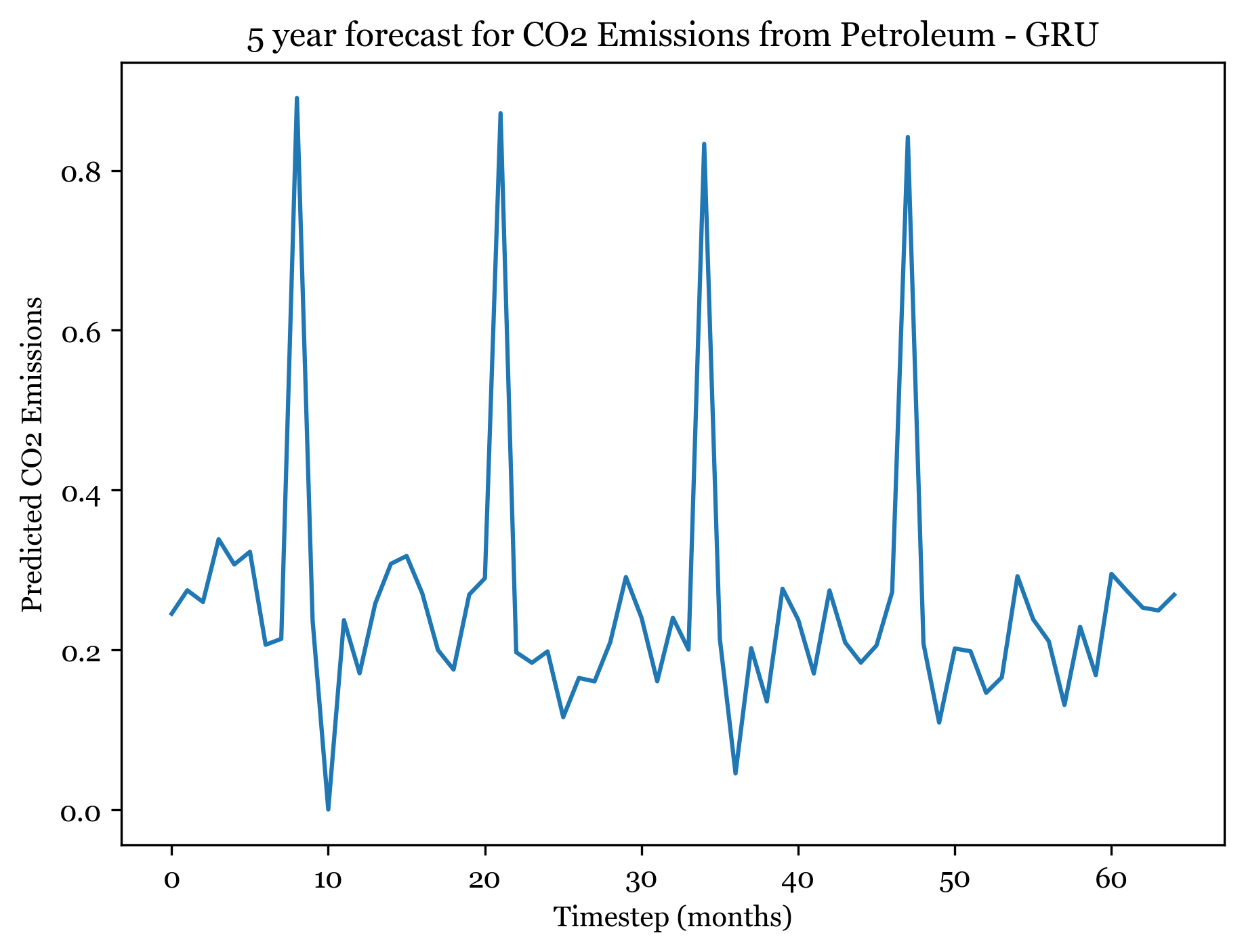
Model 3 - LSTM
Model Architecture
Model: "sequential_11"
_________________________________________________________________
 Layer (type)                Output Shape              Param #
=================================================================
 lstm_3 (LSTM)               (None, 3)                 60

 dense_11 (Dense)            (None, 1)                 4

=================================================================
Total params: 64
Trainable params: 64
Non-trainable params: 0
_________________________________________________________________
Plot training and validation loss
1/2 [==============>...............] - ETA: 0s2/2 [==============================] - 0s 2ms/step
1/1 [==============================] - ETA: 0s1/1 [==============================] - 0s 19ms/step
(51, 9, 1) (51,) (51,) (5, 9, 1) (5,) (5,)
(51,) (51,)
0.03467253
0.01929382
Train MSE = 0.03467 RMSE = 0.18621
Test MSE = 0.01929 RMSE = 0.13890
Forecasting - next 5 years (60 months)
1/1 [==============================] - ETA: 0s1/1 [==============================] - 0s 20ms/step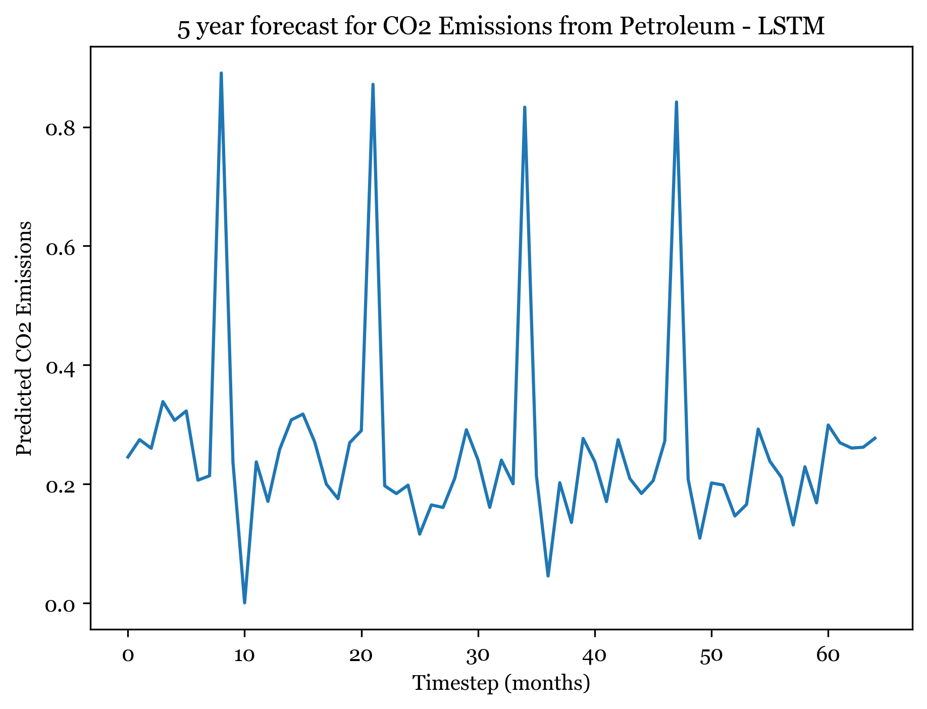
Discussion
For predicting CO2 emissions from petroleum, the training RMSE are:
1) RNN - 0.18713
2) GRU - 0.18709
3) LSTM - 0.18830
And the test RMSE are:
1) RNN - 0.09508
2) GRU - 0.14254
3) LSTM - 0.13025
Thus, the GRU model minimized RMSE for training predictions, while the RNN model minimized RMSE for test predictions. However, the RNN model may suffer from data leakage so the GRU model is likely the best model for predicting natural gas CO2 emissions going forward. Regularization improved the model performance.
Forecasting here worked better than expected. For all three models I forecasted the next 5 years (60) months, and the forecasted plots appear to mimic the seasonality and spikes of the previous 30 years. Across all three models, the first 4 years are well forecasted and display the expected spikes in emissions during the summer. However, by year 5 forecast weakens and the nuance and variation in the trend is smaller.
The SARIMA(0,1,1)(1,1,1) forecast shared the same seasonality, but exhibited a slight downwards trend across all 5 years. The ANN models exhibit no trend (only seasonality). The RMSE from the ARIMA model was 0.04678813, only slightly smaller than the ANN RMSE. The RNN had an RMSE of 0.09508, so with more model tuning could likely outperform the ARIMA model.
Comparison of Deep Learning to Traditional TS Models
In this analysis, I used 3 types of Artificial Neural Networks (ANN) to predict CO2 emissions across 4 different fuel sources: coal, hydrogen gas, natural gas, and petroleum. The goal here was to better understand which fuel sources contribute the most to climate change as well as understand trends for how their usage/consumption is changing over time. I performed a similar analysis in the ARMA/ARIMA/SARIMA Models section. Above, I compared the RMSE results and forecast results of each ANN to the ARMA/ARIMA/SARIMA results but to recap: the traditional time series models underwent significant hyperparameter tuning and model tuning in order to achieve optimal results and minimize RMSE. The ANNs implemented above were simple neural networks with minimal layers, to explore how neural networks can be used in time series analysis. Model tuning was performed, but the NNs could be further robustly tuned to experiment wtih different numbers of recurrent_hidden_units, epochs, activation functions, layers, learning rates, etc. At baseline, the neural networks were able to achieve training RMSEs of around 0.18 across all models and test RMSEs between 0.03 and 0.09. This rivals traditional models after extensive optimization, indicating that the neural networks are far superior models for time series analysis. Recurrent Neural Networks, Gated Recurrent Unit networks, and Long-Short Term Memory networks are all specifically designed to handle sequential data (such as time series) and can handle complex relationships in data better than traditional methods. They are probably better suited for handling multivariate data that a VAR model would use, while traditional time series models do perform well on univariate data like we have here. Additionally, traditional time series models are easy to interpret - whereas neural networks are more convoluted and opaque in their processes and are thus difficult to interpret beyond model fit metrics.
However, both model types performed well in the task of predicting CO2 emissions by source. In forecasting, the ARMA/ARIMA/SARIMA models were able to capture both trend and seasonality for 5 years, while the neural networks performed spectacularly for 4 years and then faltered for year 5 predictions. NN forecasting also didn’t do a great job forecasting overall trend (increases or decreases in CO2 emissions), even though they captured month to month spikes in emissions quite well.
Overall, both types of models can be useful depending on the data, and experimenting with both in order to achieve the optimal forecasting model is a good practice when dealing with any time series data.
Source code for the above analysis: Github